Prediction Intervals

Summary

A prediction interval provides a range of values that a future individual observation will lie between, with a certain probability.

Prediction intervals are ranges that estimate the future individual observations to lie with a certain probability. These intervals are used in statistical modelling and machine learning to represent the uncertainty in predictions. This range differs from a confidence interval, which estimates the range of a population parameter rather than future observations.

Probability Distribution

Derivation

Examples

Normal Distribution

Problem

The list below shows aresenic concentrations (ppb) collected every two months at two groundwater monitoring wells:

Summary statistics show year 4 has a higher sample mean and lower variance:

apply(df, 2, \(x) c("mean" = mean(x), "sd" = sd(x)))

Is there evidence of contamination for the compliance well in year 4?

Theoretical

1. $\bar{x}\sim \mathcal{N}\left(\mu ,\frac{1}{\sqrt{n}}\right)$
2. $x\sim \mathcal{N}\left(\mu ,1+\frac{1}{n}\right)$

$$\begin{array}{rl}{y}_{n+1}& \sim \mathcal{N}\left(\mu ,\sigma \right)\\ \bar{y}& \sim \mathcal{N}\left(\mu ,\frac{\sigma }{\sqrt{n}}\right)\\ y_{n+1}-\bar{y}& \sim \mathcal{N}\left(\mathrm{mean}\left(\mu -\mu \right),\sqrt{{\sigma }^2+\frac{{\sigma }^2}{\mathrm{n}}}\right)\\ & \text{Assume the mean value and next value are independent}\\ & \sim \mathcal{N}\left(0,\mathrm{var}\left(\sigma \sqrt{1+\frac{1}{n}}\right)\right)\\ \frac{y_{n+1}-\bar{y}}{\sqrt{1-\frac{1}{\sqrt{n}}}}& \sim \mathcal{N}\left(0,\sigma \right)\\ ⟹y_{n+1}& \in \bar{y}\pm z_{\alpha }\sqrt{1+n}\end{array}$$

If $\sigma$ is not known (which is likely), it can be shown ²:

$$\frac{y_{n+1}}{s}\sim t_{\alpha ,n-1}$$

This gives us:

$$\bar{y}\pm s_y\cdot t_{\alpha }\sqrt{1+\frac{1}{n}}$$

This, however, is only a one step prediction. To take multiple predictions forward is yet more work. The 95% probability would correspond to the product of both observations and the interval would have to be adjusted accordingly. This is complicated to implement, so instead we use the Bonferroni Correction. Broadly speaking, the Bonferroni Correction offsets the fallacy of multiple comparisons by dividing the quantile by the number of comparisons, so instead the interval would be given by ³:

The help for EnvStats suggests this method will be more conservative:

Approximate Method Based on the Bonferroni Inequality (method="Bonferroni")

As shown above, when k=1k=1, the value of KK is given by Equation (8) or Equation (9) for two-sided or one-sided prediction intervals, respectively. When k>1k>1, a conservative way to construct a (1−α∗)100%(1−α∗)100% prediction interval for the next kk observations or averages is to use a Bonferroni correction (Miller, 1981a, p.8) and set α=α∗/kα=α∗/k in Equation (8) or (9) (Chew, 1968). This value of KK will be conservative in that the computed prediction intervals will be wider than the exact predictions intervals. Hahn (1969, 1970a) compared the exact values of KK with those based on the Bonferroni inequality for the case of m=1m=1 and found the approximation to be quite satisfactory except when nn is small, kk is large, and αα is large. For example, Gibbons (1987a) notes that for a 99% prediction interval (i.e., α=0.01α=0.01) for the next kk observations, if n>4n>4, the bias of KK is never greater than 1% no matter what the value of kk.

However, prediction intervals will always be too narrow ⁴, so using the Bonferroni correction is no less accurate and it is simpler to implement (even if libraries do it, we must verify our results). The EnvStats package includes both the bonferroni method and the exect method, for more information on the exact method see ⁵. The formula for the exact method is included below, but is not needed, this formula is adapted from ⁶:

Putting this all together, in R:

df <- data.frame(
    y1 = c(12.6, 30.8, 52.0, 28.1),
    y2 = c(33.3, 44.0, 3.0,  12.8),
    y3 = c(58.1, 12.6, 17.6, 25.3),
    y4 = c(48.0, 30.3, 42.5, 15.0),
    y5 = c(47.6,  3.8,  2.6, 51.9))

y <- background <- c(df$y1, df$y2, df$y3)
compliance <- c(df$y3, df$y4)

pred_int_normal_population <- function(y, k, conf_level) {
    n <- length(y)
    a <- (1-conf_level) / 2
    mean(y) + c(1, -1) * sd(y) * qt(p = a / k, df = n - 1) * sqrt(1 + 1/n)
}

pred_int_normal_population(y,            k = 4, conf_level = 0.95)
## EnvStats::predIntNorm(x = y, n.mean = 1, k = 4, conf.level = 0.95)

[1] -25.54131  80.57465

Prediction Intervals of Other Models

$${\hat{y}}_{T+h|T}\pm t_{\alpha /k}{\hat{\sigma }}_h,$$

where:

• ${\hat{\sigma }}_h=K\hat{\sigma }$
• $\hat{\sigma }=\sqrt{\frac{1}{T-K-M}{\sum }_{t=1}^T{e}_t^2}$
  • $\approx$ sd(y-yhat)

Different K values can be solved:

This will be handled for us by the forecast or EnvStats package.

Using predict

It's also possible to fit a stationary linear model, which is a mean-value time series, and call the predict function:

## y is the variable of concern
y <- rnorm(10)

## Generate some indices
x <- 1:10
 
## Fit a line
## The slope should be zero, so the model will fit only intercept
model <- lm(y ~ 0)

# Now create a new data frame with the new x values
new_x <- data.frame(x = 11:14)

# Use the 'predict' function to make prediction
predictions <- predict(model, new_x, interval = "prediction")

print(predictions)

EnvStats Package

df <- data.frame(
    y1 = c(12.6, 30.8, 52.0, 28.1),
    y2 = c(33.3, 44.0, 3.0,  12.8),
    y3 = c(58.1, 12.6, 17.6, 25.3),
    y4 = c(48.0, 30.3, 42.5, 15.0),
    y5 = c(47.6,  3.8,  2.6, 51.9))


library(EnvStats)
EnvStats::predIntNorm(
            c(df$y1, df$y2, df$y3), # Flatten the values
            n.mean = 1,             # 1 for 1 observation
            k = 4,                  # Make 4 Future Predictions
            conf.level = 0.95       # The probability for the interval
            )

Results of Distribution Parameter Estimation
--------------------------------------------

Assumed Distribution:            Normal

Estimated Parameter(s):          mean = 27.51667
                                 sd   = 17.10119

Estimation Method:               mvue

Data:                            c(df$y1, df$y2, df$y3)

Sample Size:                     12

Prediction Interval Method:      Bonferroni

Prediction Interval Type:        two-sided

Confidence Level:                95%

Number of Future Observations:   4

Prediction Interval:             LPL = -25.54131
                                 UPL =  80.57465

Each of the values [48.0, 30.3, 42.5, 15.0] is within $\left(-26,81\right)$ so there is insufficient evidence to conlcude there was contamination in year 4.

If we wanted to look over the next 8 years, the prediction interval would get wider:

library(EnvStats)
x = EnvStats::predIntNorm(
            c(df$y1, df$y2, df$y3), # Flatten the values
            n.mean = 1,             # 1 for 1 observation
            k = 8,                  # Make 4 Future Predictions
            )


lpl <- x$interval$limits[1]
upl <- x$interval$limits[2]
obs <- c(df$y4, df$y5)
if (sum(lpl < obs & obs < upl)) {
  print("No Evidence")
} else {
  cat("Evidence to Reject H0")
}

Results of Distribution Parameter Estimation
--------------------------------------------

Assumed Distribution:            Normal

Estimated Parameter(s):          mean = 27.51667
                                 sd   = 17.10119

Estimation Method:               mvue

Data:                            c(df$y1, df$y2, df$y3)

Sample Size:                     12

Prediction Interval Method:      Bonferroni

Prediction Interval Type:        two-sided

Confidence Level:                95%

Number of Future Observations:   8

Prediction Interval:             LPL = -32.47117
                                 UPL =  87.50450

Log-Normal Distribution

All values are strictly positive, this may suggest a log-normal distribution is more appropriate.

Theoretical

This can be solved by using a log transform and then exponentiating the intervals:

pred_int_log_normal_population <- function(y, k, conf_level) {
    n <- length(y)
    a <- (1-conf_level) / 2

    y  <- log(y)
    SE <- sd(y) * sqrt(1 + 1/n)
    t  <- qt(p = a / k, df = n - 1)
    intervals <- mean(y) + c(1, -1) *  t * SE
    exp(intervals)
}

1.679715  278.144795

EnvStats

EnvStats::predIntLnorm(x = y, k = 4, conf.level = 0.95)

Results of Distribution Parameter Estimation
--------------------------------------------

Assumed Distribution:            Lognormal

Estimated Parameter(s):          meanlog = 3.0733829
                                 sdlog   = 0.8234277

Estimation Method:               mvue

Data:                            y

Sample Size:                     12

Prediction Interval Method:      Bonferroni

Prediction Interval Type:        two-sided

Confidence Level:                95%

Number of Future Observations:   4

Prediction Interval:             LPL =   1.679715
                                 UPL = 278.144795

> 

Built-in Function: Population Value From Sample Value

Linear Regression

Prediction Intervals of Linear Models

Examples

Theoretical: Next Value from a Model

The prediction interval for a linear value is given by ⁸:

$${\hat{y}}_h\pm t_{(1-\alpha /2,n-2)}\times \sqrt{MSE\times \left(1+\frac{1}{n}+\frac{(x_i-\bar{x}{)}^2}{{\sum }_{j=1}^n(x_j-\bar{x}{)}^2}\right)}$$

set.seed(123) # Ensuring reproducibility
n = 100 # Defining n
x = 1:n
m = 3
err = rnorm(n) # Creating error term
y = m * x + err # Generating y
data = data.frame(x = x, y = y) # Creating a data frame

x_i = 7 # This the point we are interested in

# Calculate prediction interval
fit = lm(y ~ x, data) # Fitting the model
predict(fit, newdata = list(x = x_i), interval = "predict", level = 0.95)

# Calculate prediction interval by hand
SE = summary(fit)$sigma # Extract the standard error from the model fit
hat_y_i = coef(fit)["(Intercept)"] + coef(fit)["x"] * x_i # Manual prediction using the model coefficients
t_val = qt(p = 0.975, df = n - 2) # t-value for 95% confidence level with n - 2 df [fn_df]
pred_int = hat_y_i + c(fit = 0, lwr = -1,  upr = 1) * SE * sqrt(1 + 1/n + (x_i - mean(x))^2 / (n-1)*sd(x)) * t_val # Prediction Interval

# Results
pred_int


## footnotes
## [fn_df] Each parameter in the model consumes a degree of freedom
## 1 for intercept + 1 for slope
## See generally ch. 2 and 3 of
## Bingham, N. H., and John M. Fry. Regression: Linear Models in Statistics. Springer Undergraduate Mathematics Series. London ; New York: Springer, 2010.

     fit      lwr      upr
20.98117 19.13687 22.82548
     fit      lwr      upr 
20.98117 19.13687 22.82548 

In the interest of completeness, the SE could also be calculated from first principles:

## Define a function to get Standard Error from linear regression
linear_SE <- function(model) {
    ## Residual Sum of Squares (RSS)
    ## Could also do
    ## sum((y - predict(model))^2)
    rss = sum(model$residuals^2)

    # Degrees of Freedom
    df = n - length(coef(model))

    # Compute Standard Error (SE)
    SE = sqrt(rss/df)

    ## Should be equal to
    ## Compare with SE from summary
    ## SE = summary(model)$sigma
}

Built-in Function: Next Value from a Model

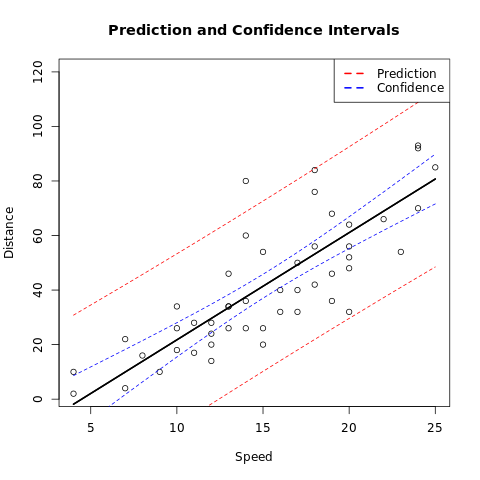
Base Plots

# Build the linear mod
m <- lm(dist ~ speed, data = cars)

# Create a Prediction and Confidence interval for new data on the mod
alpha <- 0.95
newdata <- list(speed = cars$speed)
make_pred <- function(type) {
    predictions = predict(m, newdata = newdata, interval = type, level = alpha)
    data.frame(speed = cars$speed, predictions)
}

# Create datafra
pred_df <- make_pred("prediction")
conf_df <- make_pred("confidence")

# Plot the Da
plot(dist ~ speed,
    data = cars,
    xlim = range(speed),
    ylim = range(dist),
    main = "Prediction and Confidence Intervals",
    xlab = "Speed",
    ylab = "Distance"
)

# Add the prediction interv
cols = c(pred = "red", conf = "blue")
with(pred_df, {
    lines(speed, fit, lwd = 2)
    lines(speed, lwr, lty = 2, col = cols["pred"])
    lines(speed, upr, lty = 2, col = cols["pred"])
})
# Add the Confidence Interv
with(conf_df, {
    lines(speed, fit, lwd = 2)
    lines(speed, lwr, lty = 2, col = cols["conf"])
    lines(speed, upr, lty = 2, col = cols["conf"])
})

## Add a lege
legend("topright",
    legend = c("Prediction", "Confidence"),
    lty = c(2, 2), col = cols, lwd = 2
)

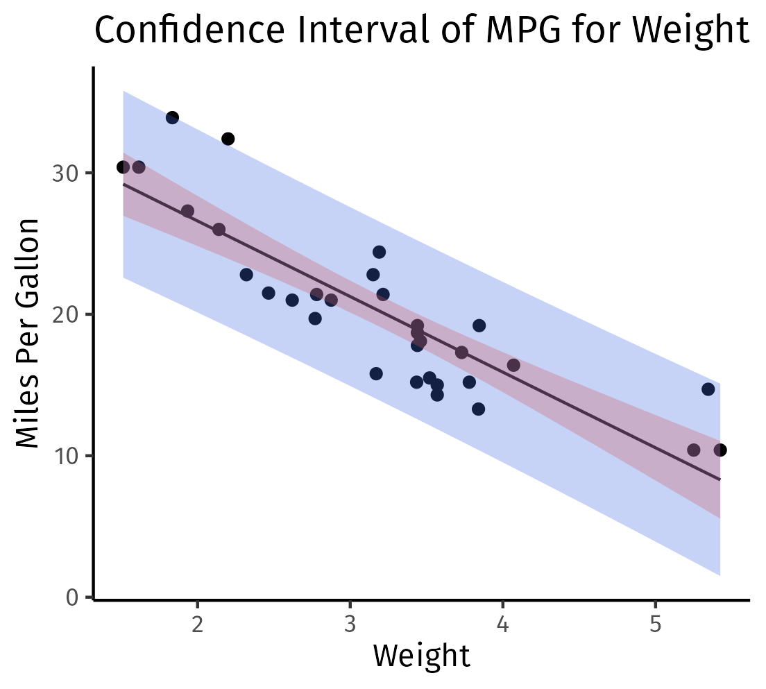
Tidyverse and GGPlot

# Load necessary librari
library(ggplot2)
library(tidyverse)
library(broom)

# Fit a linear model (Predict mpg using a single predictor, e.g., w
fit <- lm(mpg ~ wt, data=mtcars)

newdata <- data.frame(wt = seq(min(mtcars$wt), max(mtcars$wt), len=100))

conf_int <- predict(fit, newdata = newdata, interval = 'confidence') %>%
  as_tibble() %>%
  mutate(wt = newdata$wt)

pred_int <- predict(fit, newdata = newdata, interval = 'prediction') %>%
  as_tibble() %>%
  mutate(wt = newdata$wt)

# Making ggplot including confidence interv
ggplot() +
  geom_point(data = mtcars, aes(x=wt, y=mpg)) +
  geom_line(data=conf_int, aes(x=wt, y=fit)) +
  geom_ribbon(data=pred_int, aes(x = wt, y = fit, ymin=lwr, ymax=upr), alpha=0.3, fill = "royalblue") +
  geom_ribbon(data=conf_int, aes(x = wt, y = fit, ymin=lwr, ymax=upr), alpha=0.3, fill = "indianred") +
  labs(title="Confidence Interval of MPG for Weight", x="Weight", y="Miles Per Gallon") +
  theme_classic()

ggsave("../assets/images/confidence_and_prediction_interval.png")

Bootstrap

A simple bootstrap for the prediction interval of a linear model is included below. Note this assumes constant variance across the model, see ⁷ for a more detailed walkthrough of bootstrapping prediction intervals.

pred_vals <- replicate(10 ^ 4, {
  n = nrow(my_cars)
  form <- dist ~ speed
  ## Re-Sample the cars with replacement
  s = sample(1:n, replace = TRUE)
  cars_boot <- my_cars[s,]

  ## Fit a Linear Model
  mod <- lm(form, cars_boot)

  inter <- coef(mod)[1]
  slope <- coef(mod)[2]

  ## Get the predicted value at x=10
  pred_val <- 10 * slope + inter
  
  ## Find the residuals of the bootstrap model
  residuals <- resid(mod)
  
  ## Randomly select one of the residuals
  selected_resid <- sample(residuals, 1)
  
  ## Add the selected residual to the predicted value
  pred_val_selected_resid <- pred_val + selected_resid

  pred_val_selected_resid

})

hist(pred_vals)

quantile(pred_vals, c(0.025, 0.975))

## Confidence Interval
form <- dist ~ speed
fit <- lm(form, my_cars)
stats::predict(
  fit,
  newdata = list(speed = 10),
  interval = "prediction",
  levels = c(0.025, 0.975)
)

Derivation

We define Linear regression for matrices $\mathbf{X}$ and $\mathbf{Y}$ as:

$$\mathbf{Y}=\mathbf{BX}$$

The closed form solution for $\mathbf{X}$ is:

$$B={\left(X^{\mathrm{T}}X\right)}^{-1}{X}^{\mathrm{T}}Y$$

We define:

• Population Slope
  • $\beta$
• Sample Slope
  • $\mathbf{B}$

In the context of linear regression both $\beta$ and $\mathbf{B}$ represent matrices of coefficients. If $\mathrm{size}\left(Y\right)=n\times 1$ then the coefficient matrices will simply be vectors.

As a first step, we must solve the covariance of the weights matrix, before reading further make sure to review Covariance.

To begin, recall that the sum of variance in two vectors is the sum of the variance in each plus double the covariance:

$$\begin{array}{rl}\mathrm{var}\left(X-Y\right)& =\sum _{i=1}^n\left[{\left(x-y-\left(\bar{x}-\bar{y}\right)\right)}^2\right]\\ & =\sum _{i=1}^n\left[x^2-2xy+y^2-2x\bar{x}+2x\bar{y}+2\bar{x}y+2y\bar{y}+{\bar{x}}^2-2\bar{x}y+{\bar{y}}^2\right]\\ & =\sum _{i=1}^n\left[x^2-2x\bar{x}+{\bar{x}}^2\right]-2\sum _{i=1}^n\left[\left(x-\bar{x}\right)\left(y-\bar{y}\right)\right]+\sum _{i=1}^n\left[y^2-2y\bar{y}+{\bar{y}}^2\right]\\ & =\mathrm{var}\left(x\right)-2\mathrm{cov}\left(x,y\right)+\mathrm{var}\left(y\right)\end{array}$$

We can decompose the weights matrix to include the population weights and the noise in the observation:

$$\begin{array}{rl}B& ={\left(X^{\mathrm{T}}X\right)}^{-1}{X}^{\mathrm{T}}Y\\ & ={\left(X^{\mathrm{T}}X\right)}^{-1}{X}^{\mathrm{T}}\left(X\beta +\epsilon \right)\\ & ={\left(X^{\mathrm{T}}X\right)}^{-1}{X}^{\mathrm{T}}X\beta +{\left(X^{\mathrm{T}}X\right)}^{-1}{X}^{\mathrm{T}}\epsilon \\ & ={\left(X^{\mathrm{T}}X\right)}^{-1}\left(X^{\mathrm{T}}X\right)\beta +{\left(X^{\mathrm{T}}X\right)}^{-1}{X}^{\mathrm{T}}\epsilon \\ & =\beta +{\left(X^{\mathrm{T}}X\right)}^{-1}{X}^{\mathrm{T}}\epsilon \end{array}$$

This can be used to show the weights matrix is an unbiased estimator of the population weights:

$$\begin{array}{rl}\mathrm{E}\left(B\right)& =\mathrm{E}\left[\beta +{\left(X^{\mathrm{T}}X\right)}^{-1}{X}^{\mathrm{T}}\epsilon \right]\\ & =\mathrm{E}\left[\beta \right]+\mathrm{E}\left[{\left(X^{\mathrm{T}}X\right)}^{-1}{X}^{\mathrm{T}}\epsilon \right]\\ & =\beta +{\left(X^{\mathrm{T}}X\right)}^{-1}{X}^{\mathrm{T}}\mathrm{E}\left[\epsilon \right]\\ & \text{The expected value of }\epsilon \text{ is 0}\\ & =\beta +{\left(X^{\mathrm{T}}X\right)}^{-1}{X}^{\mathrm{T}}0\\ & =\beta \end{array}$$

Re-arranging, this gives the difference between the sample and population weights matrix:

$$\begin{array}{rl}B-\mathrm{E}\left[B\right]& =B-\beta \\ & =\beta +{\left(X^{\mathrm{T}}X\right)}^{-1}{X}^{\mathrm{T}}\epsilon -\beta \\ & ={\left(X^{\mathrm{T}}X\right)}^{-1}{X}^{\mathrm{T}}\epsilon \\ {\left(B-\mathrm{E}\left[B\right]\right)}^{\mathrm{T}}& ={\left({\left(X^{\mathrm{T}}X\right)}^{-1}{X}^{\mathrm{T}}\epsilon \right)}^{\mathrm{T}}\\ & ={\left(X^{\mathrm{T}}\epsilon \right)}^{\mathrm{T}}{\left({\left(X^{\mathrm{T}}X\right)}^{-1}\right)}^{\mathrm{T}}\\ & =\epsilon X{\left({\left(X^{\mathrm{T}}X\right)}^{\mathrm{T}}\right)}^{-1}\\ & =\epsilon X{\left(X^{\mathrm{T}}X\right)}^{-1}\end{array}$$ Finally, we can solve the covariance matrix in terms of the population standard deviation: $$\begin{array}{rl}\mathrm{cov}\left(B\right)& =\mathrm{E}\left[\left(B-E\left[B\right]\right){\left(B-E\left[B\right]\right)}^{\mathrm{T}}\right]\\ & ={\left(X^{\mathrm{T}}X\right)}^{-1}{X}^{\mathrm{T}}\mathrm{E}\left[\epsilon {\epsilon }^{\mathrm{T}}\right]X{\left(X^{\mathrm{T}}X\right)}^{-1}\\ & ={\left(X^{\mathrm{T}}X\right)}^{-1}{X}^{\mathrm{T}}{\sigma }^{2}IX{\left(X^{\mathrm{T}}X\right)}^{-1}\\ & ={\sigma }^2{\left(X^{\mathrm{T}}X\right)}^{-1}{X}^{\mathrm{T}}X{\left(X^{\mathrm{T}}X\right)}^{-1}\\ & ={\sigma }^2{\left(X^{\mathrm{T}}X\right)}^{-1}\end{array}$$

The confidence interval depends on the variance in model predictions:

$$\begin{array}{rl}\mathrm{var}\left({\hat{y}}_0\right)& =\mathrm{E}\left[\left(X_{0}B-\mathrm{E}\left[X_{0}B\right]\right){\left(X_{0}B-\mathrm{E}\left[X_{0}B\right]\right)}^{\mathrm{T}}\right]\\ & =X_0\mathrm{E}\left[\left(B-\mathrm{E}\left[B\right]\right){\left(B-\mathrm{E}\left[B\right]\right)}^{\mathrm{T}}\right]X_0^{\mathrm{T}}\\ & =X_0\mathrm{cov}\left(B\right)X_0^{\mathrm{T}}\\ & ={\sigma }^2{X}_0{\left(X^{\mathrm{T}}X\right)}^{-1}{X}_0^{\mathrm{T}}\end{array}$$

This is the standard error used to solve the confidence interval.

The prediction interval is the standard error in the residuals, which is given by:

$$\begin{array}{rl}\mathrm{var}\left(y_0-{\hat{y}}_0\right)& =\mathrm{var}\left(y_0\right)-2\mathrm{cov}\left(y_0,{\hat{y}}_0\right)+\mathrm{var}\left({\hat{y}}_0\right)\\ & =\mathrm{var}\left({\epsilon }_0\right)-2\mathrm{cov}\left({\epsilon }_0,{\hat{y}}_0\right)+\mathrm{var}\left({\hat{y}}_0\right)\\ & =\mathrm{var}\left({\epsilon }_0\right)-2X_0\mathrm{cov}\left({\epsilon }_0,B\right)+\mathrm{var}\left({\hat{y}}_0\right)\\ & \\ & \text{In Linear regression, the variance of the error}\\ & \text{is independent of the slope, so covariance is 0 }\\ & \\ & =\mathrm{var}\left({\epsilon }_0\right)-0+\mathrm{var}\left({\hat{y}}_0\right)\\ & ={\sigma }^2+{\sigma }^2{X}_0{\left(X^{\mathrm{T}}X\right)}^{-1}{X}_0^{\mathrm{T}}\\ & ={\sigma }^2\left(1+X_0{\left(X^{\mathrm{T}}X\right)}^{-1}{X}_0^{\mathrm{T}}\right)\end{array}$$

Using this we can solve the confidence interval with:

$$\bar{x}\pm z_{\alpha }\mathrm{SE}$$

Of course, we don't know $\sigma$ so we use t, it can be shown : ¹⁰

$$\frac{\beta -\hat{\beta }}{\hat{\sigma }}=\frac{\mathcal{N}\left(0,{\mathbf{C}}^{-1}\right)}{\sqrt{{\chi }_{n-p}^2}/(n-p)}\sim t_{n-p}$$

which implies

• confidence interval:

  $$\mathbf{Y}\in \mathbf{B}\pm t_{\alpha ,(n-p)}\sqrt{\mathrm{var}\left(\hat{\mathbf{Y}}\right)}$$

• prediction interval:

  $${\mathbf{Y}}_i\in \mathbf{B}\pm t_{\alpha ,(n-p)}\sqrt{\mathrm{var}\left(\mathbf{Y}-\hat{\mathbf{Y}}\right)}$$

Where $\mathbf{C}={\left({\mathbf{X}}^{\mathrm{T}}\mathbf{X}\right)}^{-1}$ is the control matrix.

Footnotes