Test Training Splits
Data Splits
Test Training Split
Cross-Sectional Data
When modelling data, we must use performance charactacteristics to fit a given model and we must also choose which model is most appropriate, consider the visualisation below 1:
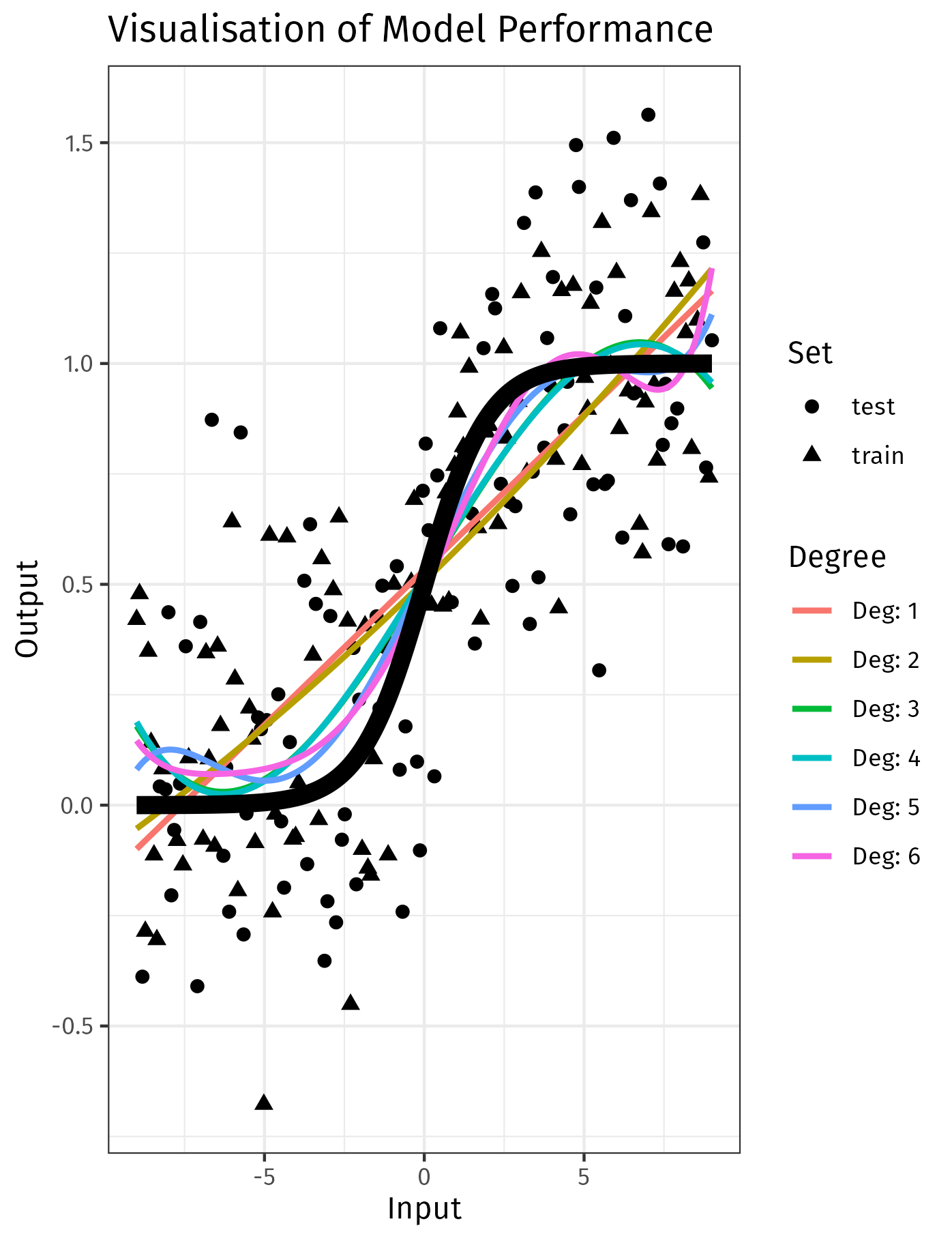
In that visualisation, models of a higher degree may fit the training data closer, but this occurs at the expense of general performance, i.e. validation error.
Typically we split data into three sets:
- Training
- Fit the model to this data
- Validation
- After fitting the model, measure the performance on this set of data
- This can be used to compare multiple models to determine which model was most accurate
- Testing
- After deciding on the best model, evaluate the performance on this data in order to estimate the amount of error in the model for unseen data.
There are other methods of estimating testing error AIC, BIC and cross validation, these aren't covered in this subject, see generally §§5.1, 6.1 of 2.
Cross-Sectional Data
Cross-Sectional Data
Firstly, set a seed for reproducibility, this can make debugging much easier 3:
set.seed(123)
data <- iris
Now, you need to create a random permutation of the row indices. This allows you to randomly shuffle the data:
index <- sample(1:nrow(data), nrow(data))
Use these indices to shuffle the dataset:
data <- data[index, ]
It's common to use 70% for training, 15% for validation, and 15% for testing. There is no hard rule for this though 4:
train_index <- round(0.7 * nrow(data))
valid_index <- train_index + round(0.15 * nrow(data))
Finally, use these indices to split the data:
train_data <- data[1:train_index, ]
valid_data <- data[(train_index+1):valid_index, ]
test_data  <- data[(valid_index+1):nrow(data), ]
That's the general concept of testing and training splits. In practice it might be useful to use a dedicated library like caret, rsample or sklearn.model_selection.train_test_split in Python, these are less error prone because the logis is wrapped up in a well-tested function.
Also, be aware that splitting data this way might not maintain the original proportion of different classes especially in imbalanced type sets. For that case, you would need to do stratified sampling.
Also, be aware that this specific implemnetation did not maintain the orginial class proportions, this can be important for imabalanced datasets. When you have significant data imbalance, it may be necessary to look into other techniques such as over-sampling 5. An example of this type of situation is disease, models may simply predict all inputs as healthy when diseased observations are small in proportion.
Cross-Sectional Data
Split the data like so:
from sklearn import datasets
import sklearn
from sklearn.model_selection import train_test_split
from sklearn.preprocessing import PolynomialFeatures
from sklearn.linear_model import LinearRegression
from sklearn.pipeline import make_pipeline
from sklearn.metrics import mean_squared_error

import numpy as np

# load iris datase
iris = datasets.load_iris()

# just use the first two features (sepal length and sepal width
X = iris.data[:, :2] # pyright: ignore
y = iris.target      # pyright: ignore

# data spli
X_train_val, X_test, y_train_val, y_test = train_test_split(X, y, test_size=0.2, random_state=42)
X_train, X_val, y_train, y_val = train_test_split(X_train_val, y_train_val, test_size=0.25, random_state=42)
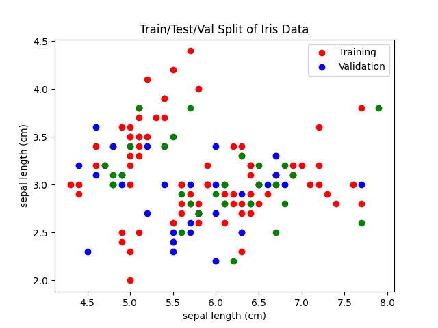
We can visualize this test traiing split:
plt.scatter(X_train[:, 0], X_train[:, 1], c="r")
plt.scatter(X_val[:, 0], X_val[:, 1], c="b")
plt.scatter(X_test[:, 0], X_test[:, 1], c="g")
plt.legend(["Training", "Validation"])
plt.title("Train/Test/Val Split of Iris Data")
plt.xlabel(iris.feature_names[0])
plt.ylabel(iris.feature_names[0])
plt.savefig("../assets/images//test_training_split_iris_example.png")
We can then fit a linear and polynomial model:
# Linear model
## Fit the model
model_linear = LinearRegression()
model_linear.fit(X_train, y_train)
## Get the Training Error
train_error_linear = mean_squared_error(
        y_train,
        model_linear.predict(X_train))
## Get the Validation Error
val_error_linear = mean_squared_error(
        y_val,
        model_linear.predict(X_val))

# Quadratic model
model_quadratic = make_pipeline(PolynomialFeatures(2), LinearRegression())
model_quadratic.fit(X_train, y_train)
## Get the Training Error
train_error_quadratic = mean_squared_error(
        y_train,
        model_quadratic.predict(X_train))
## Get the Validation Error
val_error_quadratic = mean_squared_error(
        y_val,
        model_quadratic.predict(X_val))

import json
my_dict = {
        'training': {
            'linear': round(train_error_linear, 3),
            'quadratic': round(train_error_quadratic, 3) },
        'validation': {
            'linear': round(val_error_linear, 3),
            'quadratic': round(val_error_quadratic, 3) }
        }
print(json.dumps(my_dict, indent=2))
{
  "training": {
    "linear": 0.181,
    "quadratic": 0.159
  },
  "validation": {
    "linear": 0.209,
    "quadratic": 0.202
  }
}
Do you notice how the quadratic model has a lower training error (0.159 < 0.181) but the validation error is not signifianctly lower (0.209 ≅ 0.202)? This is a common pattern with complex models, they overfit the training data and perform pooly on validation data.
Temporal Data
Summary
When fitting models to time series data, it is also necessary to partition the data. However, in time series, the data is not split randomly, rather we allocate a portion of the most recent data as validation.
It is typical to omit a test period because the omission of the most recent periods may lead compromise the accuracy of the validation error, which may lead the wrong choice of model.
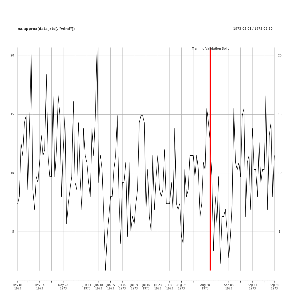
Example
Here is an example of a training/validation split applied to the EnvStats::Air.df data.
# Load required packages
library(xts)
library(EnvStats)

## Import some data as a dataframe
df <- EnvStats::Air.df

## First separate out the dates and the data
## use help(strftime) to find the format codes
index <- as.Date(rownames(df), format = "%m/%d/%Y")
data <- df

## converting df to xts
data_xts <- as.xts(df, order.by=index, format="%Y-%m-%d")

## Set split percentage
split_percent <- 0.75

## Get index to split the dataset
split_index <- round(nrow(data_xts) * split_percent)

## Create the training set
training_set_xts <- data_xts[1:split_index]

## Create the validation set
validation_set_xts <- data_xts[(split_index+1):nrow(data_xts)]

## Plot the Data
png(file = "../assets/images/validation_split_ozone_data.png",
    width = 1024,
    height = 1024,
    units = "px")
plot.xts(na.approx(data_xts[ ,"wind"]))
 split_event <- as.xts(
                       data.frame(
                                  "Training-Validation Split",
                                  order.by=as.Date(index[split_index])))
addEventLines(split_event, lwd = 5, col = "red")
dev.off()
This code for this is included in the Appendix