Introduction to the Subject

Welcome to Environmental Informatics MATH3005 !

This book represents the lecture notes for this unit, if you're taking this class, you're expected to work your way through this book and also complete the corresponding Jupyter Notebooks.

Each Topic chapter corresponds to a topic in class and will list the required readings and any lecture notes to accompany the week.

Hypothesis Testing

The focus of this class should be a revision for all students.

There is no written material for this week, rather student's should refer to the allocated readings:

Readings

Ch. 5, 6 and 7 of Open Intro Statistics ¹
Ch. 4 of Barnett, V. Environmental statistics: methods and applications. (J. Wiley, 2004).
Revision: For an introduction to R and Python see generally ² ³ ⁴ ⁵

References

https://www.openintro.org/book/os/

² https://github.com/Chris-Engelhardt/data_sci_guide/blob/master/README.md

³ https://github.com/ossu/data-science#prerequisites

⁴ https://github.com/swirldev/swirl

Biased Estimators and Sample Statistics

Variance in Terms of Expected Differences

Variance is equal to the difference between the expected square value and the expected value squared:

$Var (X) E [Var (X)] ⟹ E [\frac{1}{n} i = 1 \sum n [X_{i} - mean (X)]] = \frac{1}{n} i = 1 \sum n [(X_{i} - mean (X))^{2}] = E [\frac{1}{n} i = 1 \sum n [(X - E [X])^{2}]] The mean value is an unbiased estimator i.e. expected value of mean is the value = E [(X - E [X])^{2}] = E [X^{2} - 2 X \cdot E [X] + (E [X])^{2}] = E [X^{2}] - E [2 X \cdot E [X]] + (E [X])^{2} = E [X^{2}] - 2 (E [X])^{2} + E [X]^{2} = E [X^{2}] - E [X]^{2} = E [X^{2}] - (E [X])^{2}$

Summing Variances

$Var (X \pm Y) = E [(X \pm Y)^{2}] - E [X \pm Y]^{2} = E [X^{2} \pm 2 X Y + Y^{2}] - (E [X] \pm E [Y])^{2} = E [X^{2}] \pm 2 E [X Y] + E [Y^{2}] - (E [X] \pm E [Y])^{2} If X and Y are Independent, the Expected Value is the Product = E [X^{2}] \pm 2 E [X] E [Y] + E [Y^{2}] - (E [X] \pm E [Y])^{2} Expand the Square = E [X^{2}] \pm 2 E [X] E [Y] + E [Y^{2}] - E [X] \mp 2 E [X] E [Y] - E [Y]^{2} Cancel out the \pm and \mp = E [X^{2}] + E [Y^{2}] - E [X] - E [Y]^{2} = (E [X^{2}] - E [X]^{2}) + (E [Y^{2}] - E [Y]^{2}) = Var (X) + Var (Y)$

Note however, if $X$ and $Y$ are not independent:

$Var (X \pm Y) = Var (X) \pm 2 Cov (X, Y) + Var (Y)$

Multiplying Variance by a Constant}

$Var (a X) = E [(a X)^{2}] - E [a x]^{2} Take the constant from the left term = a^{2} E [X^{2}] - E [a x]^{2} Take the constant from the right term = a^{2} E [X^{2}] - (a E [X])^{2} = a^{2} E [X^{2}] - a^{2} E [X]^{2} a^{2} (E [X^{2}] - E [X]^{2}) a^{2} Var (X)$

Variance of a Sample Mean

Note

You may recall this:

$σ_{\overset{x}{ˉ}} = \frac{σ}{n}$

from the Central Limit Theorem ¹, we develop this idea further in the section on t-distributions.

https://en.wikipedia.org/wiki/Central_limit_theorem

Consider a sample of size $n$ , the population will have a variance $σ$ and a mean $μ$ , the sample will have a variance $s$ and a mean $\overset{x}{ˉ}$ . Many different samples could be taken, so there is a distribution of $\overset{x}{ˉ}$ values that could occur. The variance of sample means $var (\overset{x}{ˉ})$ is given by $var (x) = \frac{σ ^{2}}{n}$ , this is a part of the CLT and is shown here.

$Var (\overset{ˉ}{X}) = Var (\frac{1}{n} i = 1 \sum n [X_{i}]) Applying the product rule from earlier = (\frac{1}{n})^{2} Var (i = 1 \sum n [X_{i}]) Applying the sum rule = \frac{1}{n ^{2}} i = 1 \sum n [Var (X_{i})] The variance is already known = \frac{1}{n ^{2}} i = 1 \sum n [σ^{2}] = \frac{1}{n ^{2}} n σ^{2} = \frac{σ ^{2}}{n}$

Bessel's Correction

Suppose that the sample variance $(s)$ was given by the typical formula:

$s ⟹ E [s] ? = \frac{1}{n} i = 1 \sum n [(X_{i} - E [X])] = E [X^{2}] - E [X]^{2}$

The expected value should be $σ$ , in that sense it would be an un-biased estimator of the population mean.

The key here is to recognise that $s$ corresponds to a sample, by introducing $\overset{ˉ}{X}$ we can solve for variance in terms of expected values and the sample mean. The sample introduces the bias so it is necessary to use the sample mean.

$s^{2} ⟹ E [s^{2}] ⋆ = \frac{1}{n} i = 1 \sum n [(X_{i} - \overset{ˉ}{X})^{2}] = E [\frac{1}{n} i = 1 \sum n [(X_{i} - \overset{ˉ}{X})^{2}]] Expand the square = E [\frac{1}{n} i = 1 \sum n [X_{i}^{2} - 2 X \overset{ˉ}{X} + \overset{ˉ}{X}^{2}]]$

Note in particular, that $\overset{ˉ}{X}$ is now a form of the expression, by the CLT this will give a $Var (X) = \frac{σ ^{2}}{n}$ , this is the key insight that pulls this together, it's that very $/ n$ that accounts for the $(n - 1)$ :

$Distribute the sum = E [\frac{1}{n} i = 1 \sum n [X_{i}^{2}] - 2 \overset{ˉ}{X} i = 1 \sum n [X_{i}] + \frac{1}{n} i = 1 \sum n [\overset{ˉ}{X}^{2}]] Distribute the expectation = E [\frac{1}{n} i = 1 \sum n [X_{i}^{2}]] - 2 E [\overset{ˉ}{X}^{2}] + E [\frac{1}{n} i = 1 \sum n [\overset{ˉ}{X}^{2}]] Simplify the right-most term = E [\frac{1}{n} i = 1 \sum n [X_{i}^{2}]] - E [2 \overset{ˉ}{X}^{2}] + E [\frac{1}{n} n \overset{ˉ}{X}^{2}] = E [\frac{1}{n} i = 1 \sum n [X_{i}^{2}]] - E [2 \overset{ˉ}{X}^{2}] + E [\overset{ˉ}{X}^{2}] = E [\frac{1}{n} i = 1 \sum n [X_{i}^{2}]] - E [\overset{ˉ}{X}^{2}] The mean value is an unbiased estimator of the mean and the values are i.i.d. = E [X^{2}] - E [\overset{ˉ}{X}^{2}]$

Expected Value Squared

The expected value of $X$ is the mean value:

$E [X]^{2} = μ^{2}$

Expected Square Value

Recall the definition of Variance from earlier:

$Var (X) ≜ ⟹ E [X^{2}] E [X^{2}] - E [X]^{2} = Var (X) + E [X]^{2} = σ^{2} + μ^{2}$

Applying this to the sample mean:

$Var (\overset{ˉ}{X}) ≜ ⟹ E [\overset{ˉ}{X}^{2}] E [\overset{ˉ}{X}^{2}] - E [\overset{ˉ}{X}]^{2} = Var (\overset{ˉ}{X}) + E [\overset{ˉ}{X}]^{2} The variance of the sample mean was derived earlier = \frac{σ ^{2}}{n} + μ$

This step provides the key insight, if variance is taken on a population, there is no $n$ in the denominator

because the variance of a sample mean is different to the variance of a population statistic, the expected value of a squared sample mean is different to the expected value of a squared observation. The same $n$ from $\frac{σ}{n}$ is the same one that leands to $\frac{1}{n - 1} .$ The expected value of a squared sample mean is less than the expected value of a squared observation, because the sample mean is going to be more central.

Solving The Expected Sample Variance

$s^{2} ⟹ E [s^{2}] ? = \frac{1}{n} i = 1 \sum n [(X_{i} - \overset{ˉ}{X})^{2}] = E [X^{2}] - E [\overset{ˉ}{X}^{2}] = (σ^{2} + μ^{2}) - (\frac{σ ^{2}}{n} + μ^{2}) = \frac{n σ ^{2} - σ ^{2}}{n} = σ^{2} \frac{n - 1}{n}$

This shows that the variance formula, applied to a sample is biased. In order to correct that bias define $s_{b} = \frac{n}{n - 1} s$ like so:

$s_{b}^{2} = \frac{n}{n - 1} \frac{1}{n} i = 1 \sum n [(X_{i} - \overset{ˉ}{X})^{2}] = \frac{1}{n - 1} i = 1 \sum n [(X_{i} - \overset{ˉ}{X})^{2}]$

The expected value of this is:

$E [s_{b}^{2}] = E [\frac{n}{n - 1} s] = \frac{n}{n - 1} E [s] = \frac{n}{n - 1} \frac{n - 1}{n} σ^{2}$

The t-distribution

Often $σ$ is an unknown value, much like $μ$ . It can be shown that replacing $σ$ with $s$ results in a $t$ -distribution, so we often use that.

The t-distribution in terms of sample standard deviation

To show this, note the alternative form for $χ^{2}$ :

$χ^{2} \sim \sum z^{2} χ^{2} \sim n \frac{s ^{2}}{σ ^{2}} ⟹ s^{2} \sim n σ^{2} χ^{2}$

Applying that to the typical standardization formula:

$\frac{x - μ _{0}}{s} = \frac{x - μ _{0}}{s} = \frac{x - μ}{n σ ^{2} χ ^{2}} = \frac{x - μ}{σ n χ ^{2}} = \frac{( \frac{x - μ}{σ} )}{n χ ^{2}} = \frac{z}{n χ ^{2}}$

This right hant side is known as the t-distribution $t \sim \frac{z}{n χ ^{2}}$ , this can be verified with R:

N = 3000
n = 5
qqplot(
  rt(N, n - 1),
  rnorm(N) / sqrt(n * rchisq(N, n - 1))
)

Sampling Distributions

Recall from Biased Estimators: Variance of a Sample Mean that:

$σ_{\overset{x}{ˉ}} = \frac{σ}{n}$

Likewise:

$s_{\overset{x}{ˉ}} = \frac{s}{n}$

Simple Linear Regression

There is no written material this week, rather see the readings:

Readings

Ch. 12 of Mendenhall ¹
Ch. 8 of Open Intro Stats ²
§ 11.1, 11.2 of Probabilistic Machine Learning ³
Ch. 1 of Fry's Regression ⁴

References

¹ Mendenhall, William, Robert J. Beaver, and Barbara M. Beaver. Introduction to Probability and Statistics. 14th ed./Student edition. Boston, MA, USA: Brooks/Cole, Cengage Learning, 2013.

² https://www.openintro.org/book/os/

³ Murphy, Kevin P. Probabilistic Machine Learning: An Introduction. Adaptive Computation and Machine Learning Series. Cambridge, Massachusetts: The MIT Press, 2022.

⁴ Bingham, N. H., and John M. Fry. Regression: Linear Models in Statistics. Springer Undergraduate Mathematics Series. London ; New York: Springer, 2010.

Multiple Linear Regression

The content for this week consists primarily of readings. The subtopics included here show the derivation for Multiple Linear Regression.

Readings

Open Intro Stats Ch. 9 ¹
Mendenhall Ch. 13 ²
Further Advanced Reading
- Fry's Regression Ch. 3 ³

References

¹ https://www.openintro.org/book/os/

² Mendenhall, William, Robert J. Beaver, and Barbara M. Beaver. Introduction to Probability and Statistics. 14th ed./Student edition. Boston, MA, USA: Brooks/Cole, Cengage Learning, 2013.

RSS as a Maximum Likelihood Estimator

If the residuals of a model are expected to be normally distributed, then the paramaters should be chosen to minimize the RSS ¹.

Otherwise the choice of loss function is arbitrary.

Note

Linear Regression is simply the assumption that

$y \sim N (μ, σ)$

where $μ = m x$

Consider a linear regression:

$\overset{y}{^} = m x + b + ε$

If we presume that $ε \sim N (0, σ), \exists σ$ we could view this from a perspective of choosing a $y_{i}$ value that is normally distributed around $\overset{y}{^}_{i}$ with a variance of $σ^{2}$ .

% If we treat $\overset{y}{^}$ as a a function of $x$ the probability of seeing a value $y$ , given that this model is true and the residuals are indeed normal, is given by $pnorm (\overset{y}{^} (x), y, σ)$ , this would correspond to:

The probability of seeing any such value is:

$p (y_{i}) = \frac{1}{σ 2 π} exp (\frac{( y _{i} - y ^ _{i} ) ^{2}}{2 σ ^{2}}) = \frac{1}{σ 2 π} exp (\frac{( y _{i} - m x _{i} - b ) ^{2}}{2 σ ^{2}})$

The likelihood of seeing all the observations would be given by:

$L (y) = i \in N \prod [\frac{1}{σ 2 π} exp (- \frac{( y _{i} - y ^ _{i} ) ^{2}}{2 σ ^{2}})]$

This function only has three parameters ( $σ$ , $m$ and $b$ ), everything else is either an observed value or a constant.

What we want to do is choose values of $m$ and $b$ that maximize this likelihood for any given $σ$ :

$m, b Because log is a monotone transform: By log laws: Substituting in the probability: Drop the negative = m, b arg max (i = 1 \prod N [p (y_{i})]) = m, b arg max (lo g (i = 1 \prod N [p (y_{i})])) = m, b arg max (i = 1 \sum N [lo g (p (y_{i}))]) = m, b arg max (i = 1 \sum N [lo g (\frac{1}{σ 2 π} exp (- \frac{( y _{i} - y ^ _{i} ) ^{2}}{2 σ ^{2}}))]) = m, b arg max (\sum N [lo g (\frac{1}{σ 2 π} exp (\frac{( y _{i} - y ^ _{i} ) ^{2}}{2 σ ^{2}}))])$

$Constants can be dropped from argmin = m, b arg min (\sum N [lo g (exp (\frac{( y _{i} - y ^ _{i} ) ^{2}}{2 σ ^{2}}))]) = m, b arg min (\sum N [\frac{( y _{i} - y ^ _{i} ) ^{2}}{2 σ ^{2}}])$

$Dropping constants: = m, b arg min (i = 1 \sum N [(y_{i} - \overset{y}{^}_{i})^{2}])$

Thus, in order to maximize the likelihood of seeing any $y_{i}$ with normally distributed residuals, it is sufficient to choose values $m$ and $b$ that minimize the RSS.

Footnotes

RSS: The Residual Sum of Squares $(\sum_{i = 1}^{n} [(y_{i} - \overset{y}{^}_{i})^{2}])$

Matrix Chain Rule

If observations are recorded along rows (row-major), the following linear regression model holds and conventional definition of the partials:

$\hat{Y} \frac{\partial Y ^}{\partial W} = XW = \frac{\partial Y ^ _{ik}}{\partial W _{jk}}$

For column-major the model is:

$\hat{Y} \frac{\partial Y ^}{\partial W} = WX = \frac{\partial Y ^ _{ki}}{\partial W _{kj}}$

In either case, it will be shown that the chain rule will be:

$\frac{\partial ε}{\partial W} = \frac{\partial Y ^}{\partial W} (\frac{\partial ε}{\partial Y ^})^{T}$

Notation

The notation, $[j == l]$ is adapted from Knuth ¹ and defined as:

$δ_{j l} = I_{j l} = [j == l] = {1, j = l 0, j \neq = l$

Solving the Product Derivatives

$Y ⟹ \frac{\partial Y _{k l}}{\partial W _{ij}} = W X = \frac{\partial}{\partial W _{ij}} p = 1 \sum ncol (X) [W_{k p} X_{pl}] = p = 1 \sum ncol (X) [\frac{\partial}{\partial W _{ij}} (W_{k p} X_{pl})] = 0 + \dots \frac{\partial}{\partial W _{ij}} (W_{kj} X_{j l}) + \dots 0 = {\frac{\partial}{\partial W _{ij}} (W_{ij} X_{j l}) 0 k = i k \neq = i = [k == i] X_{j l} = δ_{ki} X_{j l}$

$Y ⟹ \frac{\partial Y _{k l}}{\partial W _{ij}} = X W = \frac{\partial}{\partial W _{ij}} p = 1 \sum ncol (X) [X_{k p} W_{pl}] = p = 1 \sum ncol (X) [\frac{\partial}{\partial W _{ij}} (X_{k p} W_{pl})] = 0 + \dots + \frac{\partial}{\partial W _{ij}} (X_{ki} W_{i l}) + 0 \dots = {\frac{\partial}{\partial W _{ij}} (X_{ki} W_{ij}) 0 j = l j \neq = l = [j == l] X_{ki} = δ_{j l} X_{ki}$

So we have:

$\frac{\partial}{\partial W _{ij}} ([W X]_{[k, l]}) \frac{\partial}{\partial W _{ij}} ([X W]_{[k, l]}) = I_{j l} X_{ki} = X_{j l} I_{ki}$

Solving the Chain Rule

For the column-major example $Y = WX$ :

$\frac{\partial ε}{\partial W _{ij}} ⟹ \frac{\partial ε}{\partial W} = q \sum [p \sum [\frac{\partial ε}{\partial Y _{pq}} \frac{\partial Y _{pq}}{\partial W _{ij}}]] q \sum [p \sum [\frac{\partial ε}{\partial Y _{pq}} \frac{\partial Y _{pq}}{\partial W _{ij}} I_{p i}]] When p \neq = i We have zero so: = q \sum [\frac{\partial ε}{\partial Y _{i q}} \frac{\partial Y _{i q}}{\partial W _{ij}}] From Matrix Identities we have: = q \sum [\frac{\partial ε}{\partial Y _{i q}} X_{j q}] Transpose X : = q \sum [\frac{\partial ε}{\partial Y ^ _{i q}} X^{T}_{q j}] By definition we have: = \frac{\partial ε}{\partial Y ^} X^{T} = \frac{\partial ε}{\partial Y ^} X^{T}$

This of course assumes column-major where the columns of $Y$ represent observations and the rows are features, in the event that these were transposed we would have

$Y_{r} X_{r} W_{r} = Y^{T} = X^{T} = W^{T}$

and hence:

$(\frac{\partial ε}{\partial W})^{T} \frac{\partial ε}{\partial W _{r}} = (\frac{\partial ε}{\partial Y ^} X^{T})^{T} = X \frac{\partial ε}{\partial Y ^}^{T} Swap for Row-Major = X_{r}^{T} \frac{\partial ε}{\partial Y ^ _{r}}$

Graham, Ronald L., Donald Ervin Knuth, and Oren Patashnik. Concrete Mathematics: A Foundation for Computer Science. 2nd ed. Reading, Mass: Addison-Wesley, 1994.

Bias Terms in Multiple Regression

Consider a matrix multiplication as shown below.

$n \times R \hat{Y} = n \times F F \times R XW$

Where:

$n$ is the sample size
$R$ is the number of columns in the output, i.e. the number of response variables (or dependent variables) being modelled
$F$ is the number of columns in the input, i.e. the number of *features (or input/independent variables)

In this representation, each of the $n$ rows of $X$ and $Y$ is an observation and the columns represent input and response variables respectively.

However, I have elected to use a column-major so let's instead represent this:

$R \times n \hat{Y} = R \times F F \times n WX$

Now each observation is a column-vector instead of a row vector.

This corresponds to a matrix form thusly:

$w_{11} w_{21} w_{31} w_{12} w_{22} w_{32} w_{13} w_{23} w_{33} x_{1} x_{2} x_{3} = w_{[1, :]} \cdot x w_{[2, :]} \cdot x w_{[3, :]} \cdot x$

note the following points:

This is a column-major representation, the $x$ vector represents a single observation and subsequent observations would become additional columns of $X$ .
- A row major representation can be acheived by transposing $^{T}$ the matrices.
- R, Julia, Octave, Wolfram and Fortran all use column-major representations
- Python, C(++), Go and Rust use a row-major representation
- It's important to get this right, languages store values in a certain pattern in memory, cutting against the grain will be less performant.
The use of sympy/octave/julia notation, whereby $w_{[1, :]}$ represents a vector composed of the first row of $W$ .

Let's now add a bias term (i.e. an intercept) so that the model reflects $y = m x + b$ from simple linear regression:

$w_{11} w_{21} w_{31} w_{12} w_{22} w_{32} w_{13} w_{23} w_{33} x_{1} x_{2} x_{3} + k_{1} k_{2} k_{3} = w_{[1, :]} \cdot x w_{[2, :]} \cdot x w_{[3, :]} \cdot x + k_{1} k_{2} k_{3} = w_{[1, :]} \cdot x + k_{1} w_{[2, :]} \cdot x + k_{2} w_{[3, :]} \cdot x + k_{3}$

The bias term could equally be expressed inside the matrix thusly:

$w_{11} w_{21} w_{31} w_{12} w_{22} w_{32} w_{13} w_{23} w_{33} k_{1} k_{2} k_{3} x_{1} x_{2} x_{3} 1 = w_{[1, :]} \cdot x + k_{1} w_{[2, :]} \cdot x + k_{2} w_{[3, :]} \cdot x + k_{3}$

That's why we don't often include a bias term when performing multiple linear regression, as it can be included as a component of the weights matrix.

More Observations

If there were $n$ observations:

$w_{11} w_{21} w_{31} w_{12} w_{22} w_{32} w_{13} w_{23} w_{33} k_{1} k_{2} k_{3} x_{11} x_{21} x_{n 1} x_{12} x_{22} x_{n 2} \dots x_{1 n} x_{2 n} x_{nn} 111 = w_{[1, :]} \cdot x + k_{1} w_{[2, :]} \cdot x + k_{2} w_{[3, :]} \cdot x + k_{3}$

Row Major

If we transformed this to a row-major representation, the 1s would now be a row of the input and the bias a row of the weights: $w_{11} w_{21} w_{31} w_{12} w_{22} w_{32} w_{13} w_{23} w_{33} k_{1} k_{2} k_{3} x_{11} x_{21} x_{n 1} x_{12} x_{22} x_{n 2} \dots x_{1 n} x_{2 n} x_{nn} 111^{T} x_{11} x_{21} x_{n 1} x_{12} x_{22} x_{n 2} \dots x_{1 n} x_{2 n} x_{nn} 111^{T} w_{11} w_{21} w_{31} w_{12} w_{22} w_{32} w_{13} w_{23} w_{33} k_{1} k_{2} k_{3}^{T} = w_{[1, :]} \cdot x + k_{1} w_{[2, :]} \cdot x + k_{2} w_{[3, :]} \cdot x + k_{3}^{T} = w_{[1, :]} \cdot x + k_{1} w_{[2, :]} \cdot x + k_{2} w_{[3, :]} \cdot x + k_{3}^{T}$

A note on Memory Layout in languages

Column major matrices are rooted in mathematical notation and conventions of linear algebra. In many textbooks and papers, 1D vectors are often treated as column vectors where convenient. This makes column-major order a natural and intuitive choice for mathematical languages where matrix operations are common. The reader may have already noted that many column-major languages are also 1-indexed, this is for a smiliar reason.

The C language was developed for systems programming, presumably row-major representation was chosen because it is consistent with how people usually layout data, there was no need to cater towards mathematical programming.

Deriving Multiple Linear Regression

Introduction

The goal here, is to maximize the probability of seeing some observation $y_{i}$ given a mean value $\overset{y}{^}_{i}$ and a constant variance $σ$

Deriving Multiple Linear Regression

Consider a multiple linear regression of the form:

$N \times 12 \hat{Y} = N \times 3 N \times 12 XW$

The bias for this model is included in the weights matrix, as shown in Bias Terms in Multiple Linear Regression.

Consider the probability of seeing an observation under the assumption:

$y_{i} ⟹ P (y_{i}) \sim N (\overset{y}{^}_{i}, σ) \propto e^{(\frac{y _{i} - y _{i} ^}{σ})^{2}}$

The goal in linear regression is to find $\hat{Y} = XW$ such that:

$W = W argmax [i = 1 \prod n (P (Y_{i}))]$

The argument $W$ which maximises the likelhood of this expression is equivalent to the the argument $W$ which minimises the rss, see Maximum Likelihood is equal to Minimum RSS

$W = W argmin [ε (W)]$

where:

$ε (W) = i = 1 \sum N j = 12 \sum 12 [(XW - Y)^{\circ 2}]$

Note that the squaring operation is elment-wise, so more conventionally:

$(ε (W))_{[ij]} = i = 1 \sum N j = 12 \sum 12 [((XW - Y)_{[ij]})^{2}]$

because $ε$ is a quadratic function:

$\frac{\partial ε}{\partial W} = 0 ⟺ W = W arg min (ε)$

Recall the Matrix Chain Rule

$\frac{\partial ε}{\partial W} \frac{\partial ε}{\partial Y ^} \frac{\partial Y ^}{\partial W} ⟹ \frac{\partial ε}{\partial W} = \frac{\partial Y ^}{\partial W} (\frac{\partial ε}{\partial Y ^})^{T} = 2 (\hat{Y} - Y) = X = 2 X^{T} (\hat{Y} - Y)$

Setting the derivative to 0:

$0 X^{T} XW W = X^{T} (XW - Y) = X^{T} XW - X^{T} Y = X^{T} Y = (X^{T} X)^{- 1} X^{T} Y$

Conclusion

So, in conclusion, if $Y = WX$ , the value for $W$ that minimises the l2 norm is ¹ ² :

$W = (X^{T} X)^{- 1} X^{T} Y$

References

"5.4 - A Matrix Formulation of the Multiple Regression Model | STAT 462." Accessed August 17, 2023. https://online.stat.psu.edu/stat462/node/132/.

s 3.1 of Bingham, N. H., and John M. Fry. Regression: Linear Models in Statistics. Springer Undergraduate Mathematics Series. London ; New York: Springer, 2010.

Confidence and Prediction Intervals

Readings

Ch. 3 Shmueli, Galit, and Kenneth C. Lichtendahl. Practical Time Series Forecasting with R: A Hands-on Guide. Second edition. Erscheinungsort nicht ermittelbar: Axelrod Schnall Publishers, 2018.
5.5 and 7.6 of https://otexts.com/fpp3/forecasting-regression.html ¹

Also available in print form: Hyndman, Rob J., and George Athanasopoulos. Forecasting: Principles and Practice. Third print edition. Melbourne, Australia: Otexts, Online Open-Access Textbooks, 2021. https://otexts.com/fpp3/#.

Introduction

This lecture provides the reader with a general understanding of how to use statistical intervals as decision rules. It explains the different techniques used including confidence intervals, prediction intervals, tolerance intervals and control charts.

In environmental monitoring, these intervals are used to compare new observation values with a standard or background value. For example, suppose that a mechanical workshop applies to refinance the mortgage on the workshop, in such cases it is common to require a soil analysis for pollutants such as sulphuric acid ². If the new measurements are greater than background values, is this evidence of an actual difference, or is it just noise?

To make an objective decision, we create a decision rule based on an interval. If the new values fall outside of the background interval, it suggests potential contamination. If the new values stay within the interval, there is insufficient evidence to suggest the higher measurements aren't caused by chance.

Footnotes

The electrolyte in lead-acid batteries used in modern cars (even in some electric cars to provide 12v to accessories)

Test Training Splits

Data Splits

Test Training Split

Cross-Sectional Data

When modelling data, we must use performance charactacteristics to fit a given model and we must also choose which model is most appropriate, consider the visualisation below ¹:

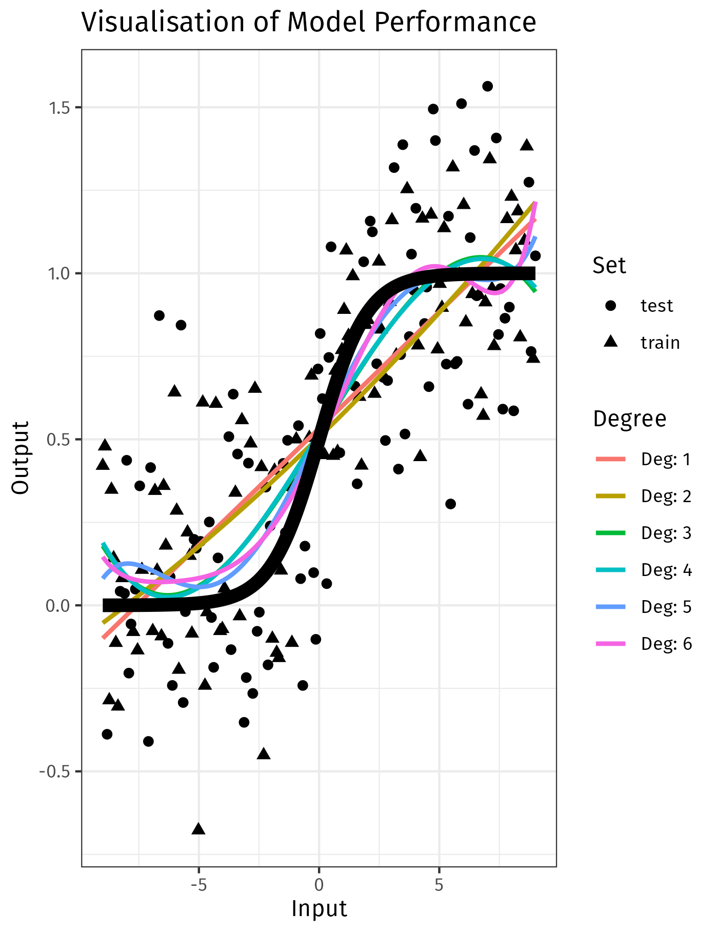
In that visualisation, models of a higher degree may fit the training data closer, but this occurs at the expense of general performance, i.e. validation error.

Typically we split data into three sets:

Training
- Fit the model to this data
Validation
- After fitting the model, measure the performance on this set of data
- This can be used to compare multiple models to determine which model was most accurate
Testing
- After deciding on the best model, evaluate the performance on this data in order to estimate the amount of error in the model for unseen data.

There are other methods of estimating testing error AIC, BIC and cross validation, these aren't covered in this subject, see generally §§5.1, 6.1 of ².

Cross-Sectional Data

Firstly, set a seed for reproducibility, this can make debugging much easier ³:

set.seed(123)
data <- iris

Now, you need to create a random permutation of the row indices. This allows you to randomly shuffle the data:

index <- sample(1:nrow(data), nrow(data))

Use these indices to shuffle the dataset:

data <- data[index, ]

It's common to use 70% for training, 15% for validation, and 15% for testing. There is no hard rule for this though ⁴:

train_index <- round(0.7 * nrow(data))
valid_index <- train_index + round(0.15 * nrow(data))

Finally, use these indices to split the data:

train_data <- data[1:train_index, ]
valid_data <- data[(train_index+1):valid_index, ]
test_data  <- data[(valid_index+1):nrow(data), ]

That's the general concept of testing and training splits. In practice it might be useful to use a dedicated library like caret, rsample or sklearn.model_selection.train_test_split in Python, these are less error prone because the logis is wrapped up in a well-tested function.

Also, be aware that splitting data this way might not maintain the original proportion of different classes especially in imbalanced type sets. For that case, you would need to do stratified sampling.

Also, be aware that this specific implemnetation did not maintain the orginial class proportions, this can be important for imabalanced datasets. When you have significant data imbalance, it may be necessary to look into other techniques such as over-sampling ⁵. An example of this type of situation is disease, models may simply predict all inputs as healthy when diseased observations are small in proportion.

Cross-Sectional Data

Split the data like so:

from sklearn import datasets
import sklearn
from sklearn.model_selection import train_test_split
from sklearn.preprocessing import PolynomialFeatures
from sklearn.linear_model import LinearRegression
from sklearn.pipeline import make_pipeline
from sklearn.metrics import mean_squared_error

import numpy as np

# load iris datase
iris = datasets.load_iris()

# just use the first two features (sepal length and sepal width
X = iris.data[:, :2] # pyright: ignore
y = iris.target      # pyright: ignore

# data spli
X_train_val, X_test, y_train_val, y_test = train_test_split(X, y, test_size=0.2, random_state=42)
X_train, X_val, y_train, y_val = train_test_split(X_train_val, y_train_val, test_size=0.25, random_state=42)

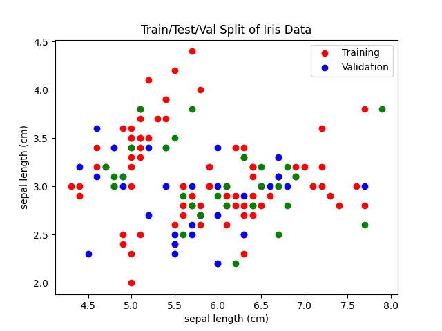
We can visualize this test traiing split:

plt.scatter(X_train[:, 0], X_train[:, 1], c="r")
plt.scatter(X_val[:, 0], X_val[:, 1], c="b")
plt.scatter(X_test[:, 0], X_test[:, 1], c="g")
plt.legend(["Training", "Validation"])
plt.title("Train/Test/Val Split of Iris Data")
plt.xlabel(iris.feature_names[0])
plt.ylabel(iris.feature_names[0])
plt.savefig("../assets/images//test_training_split_iris_example.png")

We can then fit a linear and polynomial model:

# Linear model
## Fit the model
model_linear = LinearRegression()
model_linear.fit(X_train, y_train)
## Get the Training Error
train_error_linear = mean_squared_error(
        y_train,
        model_linear.predict(X_train))
## Get the Validation Error
val_error_linear = mean_squared_error(
        y_val,
        model_linear.predict(X_val))

# Quadratic model
model_quadratic = make_pipeline(PolynomialFeatures(2), LinearRegression())
model_quadratic.fit(X_train, y_train)
## Get the Training Error
train_error_quadratic = mean_squared_error(
        y_train,
        model_quadratic.predict(X_train))
## Get the Validation Error
val_error_quadratic = mean_squared_error(
        y_val,
        model_quadratic.predict(X_val))

import json
my_dict = {
        'training': {
            'linear': round(train_error_linear, 3),
            'quadratic': round(train_error_quadratic, 3) },
        'validation': {
            'linear': round(val_error_linear, 3),
            'quadratic': round(val_error_quadratic, 3) }
        }
print(json.dumps(my_dict, indent=2))

{
  "training": {
    "linear": 0.181,
    "quadratic": 0.159
  },
  "validation": {
    "linear": 0.209,
    "quadratic": 0.202
  }
}

Do you notice how the quadratic model has a lower training error (0.159 < 0.181) but the validation error is not signifianctly lower (0.209 ≅ 0.202)? This is a common pattern with complex models, they overfit the training data and perform pooly on validation data.

Temporal Data

Summary

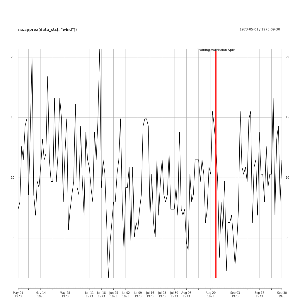
When fitting models to time series data, it is also necessary to partition the data. However, in time series, the data is not split randomly, rather we allocate a portion of the most recent data as validation.

It is typical to omit a test period because the omission of the most recent periods may lead compromise the accuracy of the validation error, which may lead the wrong choice of model.

Example

Here is an example of a training/validation split applied to the EnvStats::Air.df data.

# Load required packages
library(xts)
library(EnvStats)

## Import some data as a dataframe
df <- EnvStats::Air.df

## First separate out the dates and the data
## use help(strftime) to find the format codes
index <- as.Date(rownames(df), format = "%m/%d/%Y")
data <- df

## converting df to xts
data_xts <- as.xts(df, order.by=index, format="%Y-%m-%d")

## Set split percentage
split_percent <- 0.75

## Get index to split the dataset
split_index <- round(nrow(data_xts) * split_percent)

## Create the training set
training_set_xts <- data_xts[1:split_index]

## Create the validation set
validation_set_xts <- data_xts[(split_index+1):nrow(data_xts)]

## Plot the Data
png(file = "../assets/images/validation_split_ozone_data.png",
    width = 1024,
    height = 1024,
    units = "px")
plot.xts(na.approx(data_xts[ ,"wind"]))
 split_event <- as.xts(
                       data.frame(
                                  "Training-Validation Split",
                                  order.by=as.Date(index[split_index])))
addEventLines(split_event, lwd = 5, col = "red")
dev.off()

⁶

This code for this is included in the Appendix

Confidence Intervals

Summary

A Confidence Interval is a range of values, derived from a sample, within which the true population parameter is expected to lie. More precicely, the probability that a statistic taken from a random sample does not fall within a specified confidence interval is denoted by $α$ . In simpler terms, a confidence interval drawn from a sample, will capture the population statistic with a probability of $α$ . So in 20 samples, we would expect 19 of our $\overset{x}{ˉ}$ confidence intervals to contain the population mean $μ$ , iff the confidence intervals were 95%.

Take, for instance, a large yet finite population of fish. The average length of the fish in this population, while definite, is not possible to determine without measuring every single fish. If we were to draw 1000 samples, we'd expect that 900 of those sample means would fall within a 90% confidence interval.

It is important to be careful with the way we frame these probabilities. For example, if the data's 90% confidence interval ranged from 1 to 10, it would be incorrect to say that there's a 90% probability of the population mean falling within that range. This is because the population mean is a distinct, knowable value, it is not probalistic. The probability lies in the process of sampling. So, a more accurate statement would be, "if the population mean doesn't lie between 1 and 10, the probability of drawing such a sample was 10%".

The probability of a value within an interval, is given by the area under the curve for the corresponding distribution or PDF ¹. Confidence intervals are no different, they simply correspond to a different distribution, the sampling distribution. Revisiting the fish population experiment, if we extract a sample of these fish and compute the sample mean, the obtained value will provide a good estimate for the population mean. If multiple samples are taken and their respective means are calculated, a distribution of these sample means can be developed. The area under the curve of this distribution corresponds to the probability of observing such a sample mean, this is interval is a confidence interval.

Probability Distribution

Derivation

The Central Limit Theorem states that if sample size (n) is large enough, typically n > 30 ², the distribution of sample means will approach a $N (0, σ)$ . Since the sample mean is known follows this distribution, the confidence interval represents a specific range within this distribution, capturing a predefined proportion of random events.

Often $σ$ is an unknown value, much like $μ$ . We've seen that replacing $σ$ with $s$ results in a $t$ -distribution (see t-distribution), so confidence intervals will almost always be in terms of $t$ (unless the population variance is known, which is not common).

To derive the interval, re-arrange the z-score to represent bounds between an interval on the distribution:

$z t_{n - 1} t_{α, n - 1} s / n μ_{0} \sim \frac{x ˉ - μ _{0}}{σ _{SE}} \sim \frac{x ˉ - μ _{0}}{σ / n} \sim \frac{x ˉ - μ _{0}}{s / n} = \overset{x}{ˉ} - μ_{0} \in \overset{x}{ˉ} \pm \frac{s}{n} t_{α, n - 1}$

Examples

Theoretical: Population Mean From Sample Mean

Consider a population, we can calculate the confidence interval using the t-scores:

## Construct a populatio
population <- c(
                rep(0, 1000),
                rep(2, 1000),
                rep(30, 1000))

## Take a sampl
n    = 30
samp = sample(population, n)
xbar = mean(samp)
s = sd(samp)

alpha = 0.05  
t = abs(qt(alpha / 2, df=n-1))

# Compute the confidence limit
lower = xbar - t * (s / sqrt(n))
upper = xbar + t * (s / sqrt(n))
lower
upper

[1] 5.380967
[1] 15.81903

Note, the t.test function automatically performs a confidence interval:

## Conduct t-test and get confidence interval.
t_result = t.test(samp, conf.level = 0.95)
t_result$conf.int

If we repeat this many times, we can show that the confidence level is equal to the probability of an extreme sample:

## Construct a populatio
population <- c(
                rep(0, 1000),
                rep(2, 1000),
                rep(30, 1000))

number_of_extreme_samples <- replicate(10^3, {
    ## Take a sample
    n    = 30
    samp = sample(population, n)
    xbar = mean(samp)
    s = sd(samp)

    alpha = 0.05
    z = abs(qt(alpha / 2, df=n-1))

    ## Compute the confidence limits
    lower = xbar - z * (s / sqrt(n))
    upper = xbar + z * (s / sqrt(n))
    lower
    upper

    lower < mean(population) && mean(population) < upper
                })

mean(number_of_extreme_samples)

[1] 0.943

Bootstrapping: Confidence Intervals for Population Correlation

When a theoretical distribution for the sampling distribution is not known, it is possible to bootstrap a confidence interval. For example, consider the cars data:

speed	list
4	2
4	10
7	4
7	22
8	16
9	10
...	...

Let's assume that the R dataset is a population in and of itself. Let's take a sample use it to construct a confidence interval for the population mean. Unlike before, the formula for the confidence interval of correlation is not something most people have memorized. In this case we can bootstrap one.

The idea here is to assume that the population is an infinite repitition of the sample (acheived by sampling with replacement), we take samples from this bootstrapped population and use the quantiles of this psuedo-sampling-distribution as the confidence interval.

## Construct a populatio
population <- cars
head(cars)
n        = 30
rho <- cor(population$speed, population$dist)

take_sample <- function(p) population[sample(seq_len(nrow(population)), n), ]

## Take a sampl
samp     = take_sample(population)
rho_hat  = cor(samp$speed, samp$dist)

## Write a function to produce a sampling distributio
make_sampling_dist <- function(samp) {
    ## Bootstrap a confidence Interval for that sample
    replicate(10^3, {
        ## Take a sample with replacement (IMPORTANT)
        boot_samp <- samp[sample(n, replace = TRUE), ]

        ## Calculate the sample statistic
        cor(boot_samp$speed, boot_samp$dist)
    })
}

get_conf_interval <- function(samp, alpha) {
    lower = (1-alpha)/2
    upper = 1-lower

    quantile(make_sampling_dist(samp), c(lower, upper))
}

## Calculate the confidence interval
get_conf_interval(samp, 0.9)

       5%       95% 
0.6028544 0.8856464

Just like before, we can take this function for confidence intervals, and show that the probability of extreme samples is equal to the confidence of the interval:

## Construct a populatio
population <- cars
head(cars)
n        = 30
rho <- cor(population$speed, population$dist)

take_sample <- function(p) population[sample(seq_len(nrow(population)), n), ]

## Take a sampl
samp     = take_sample(population)
rho_hat  = cor(samp$speed, samp$dist)

## Write a function to produce a sampling distributio
make_sampling_dist <- function(samp) {
    ## Bootstrap a confidence Interval for that sample
    replicate(500, {
        ## Take a sample with replacement (IMPORTANT)
        boot_samp <- samp[sample(n, replace = TRUE), ]

        ## Calculate the sample statistic
        cor(boot_samp$speed, boot_samp$dist)
    })
}

get_conf_interval <- function(samp, alpha) {
    lower = (1-alpha)/2
    upper = 1-lower

    quantile(make_sampling_dist(samp), c(lower, upper))
}

## Calculate the confidence interval
get_conf_interval(samp, 0.9)


number_of_extreme_samples <- replicate(100, {
    ## Get a confidence Interval of a new sample
    int <- get_conf_interval(take_sample(population), 0.8)

    ## Did that confidence Interval capture the population statistic?
    int[1] < rho && rho < int[2]
})

mean(number_of_extreme_samples)

[1] 0.88

Unlike before, this value does not align with the confidence interval, that's because bootstrap methods are generally more likely to produce biased estimates when the sampling distribution is not normally distributed. This sampling distribution is right-skew, this could be inspected with:

hist(make_sampling_dist(samp))

There exist methods to overcome this limitation. ³

Linear Regression

Confidence Intervals of Linear Models

Confidence Interval of Linear Model

$Y \in B \pm t_{α, (n - p)} var (\hat{Y})$

A linear model is premised on the assumption that the data follows a Gaussian distribution, characterized by a consistent variance, while the mean is a linear function as follows:

$y_{i} ⟹ y_{i} \sim N (WX, σ) = WX + ε : ε \sim N (0, σ)$

The difference with confidence intervals for distributions that we typically use is that here, the mean is a function. This interpretation also helps to better understand the underlying assumptions of linear regression. The constant variance and Gaussian residuals aren't so much assumptions of the model but rather integral characteristics of the model itself.

Note

The confidence interval of a linear model, gives an interval through which we would expect different models to intersect. These models would correspond to different samples that we could have taken from the population.

Examples

Theoretical: Population Line From Sample Line

Consider the mtcars dataset:

head(mtcars)

                   mpg cyl disp  hp drat    wt  qsec vs am gear carb
Mazda RX4         21.0   6  160 110 3.90 2.620 16.46  0  1    4    4
Mazda RX4 Wag     21.0   6  160 110 3.90 2.875 17.02  0  1    4    4
Datsun 710        22.8   4  108  93 3.85 2.320 18.61  1  1    4    1
Hornet 4 Drive    21.4   6  258 110 3.08 3.215 19.44  1  0    3    1
Hornet Sportabout 18.7   8  360 175 3.15 3.440 17.02  0  0    3    2
Valiant           18.1   6  225 105 2.76 3.460 20.22  1  0    3    1

A multiple linear regression can be fit and a confidence interval drawn for the parameters like so:

# Compute the confidence limit
f <- mpg ~ cyl + hp + wt
mod <- lm(f, data=mtcars)

# Get the confidence intervals for the linear model
confint(mod)

                 2.5 %       97.5 %
(Intercept) 35.0915623 42.412012412
cyl         -2.0701179  0.186884238
hp          -0.0423655  0.006289293
wt          -4.6839740 -1.649972191

To predict a confidence interal on the values:

# Predict values and add confidence intervals
predict(mod, interval='confidence') |>
  head()

                         fit      lwr      upr
Mazda RX4         22.82043 21.65069 23.99016
Mazda RX4 Wag     22.01285 20.98250 23.04319
Datsun 710        25.96040 24.71014 27.21066
Hornet 4 Drive    20.93608 19.94927 21.92289
Hornet Sportabout 17.16780 15.75195 18.58365
Valiant           20.25036 19.12109 21.37962

Bootstrap

Values

# Bootstrap the linear model and calculate the coefficient estimates
bootstrap_estimates <- replicate(10^3, {
    ## Sample the data with replacement
    sample <- mtcars[sample(nrow(mtcars), replace = TRUE), ]
    ## Fit the linear model
    mod <- lm(mpg ~ cyl + hp + wt, data = sample)
    # Return the coefficients
    predict(mod, newdata = list(cyl = 4, hp = 100, wt = 2.6))
})

alpha = 0.9
lower = (1-0.9)/2
upper = 1 - lower
quantile(bootstrap_estimates, c(lower, upper))

      5%      95% 
23.43200 26.48408

Parameters

This has been ommited, the focus here is contrasting with prediction intervals. To see an example of bootstrapping the parameters, refer to the index.

Derivation

Deriving confidence intervals for linear regression is the same concept as before but I won't be showing it here. See generally the first 4 chapters of ⁴.

Footnotes

PDF: Probability Density Function

It's worth noting that extremely non-symmetric distributions will require larger sample sizes. 30 is sufficent for symmetric data though.

If we wanted we could adjust it with Fisher's z-transformation which would help reduce the bias. This is shown in the Appendix: Fisher's z-tranform. More generally there is also bias-corrected and accelerated (BCa) bootstraps, this is a method to deal with bootstraps of any skewed sampling distribution.

⁴

Bingham, N. H., and John M. Fry. Regression: Linear Models in Statistics. Springer Undergraduate Mathematics Series. London ; New York: Springer, 2010.

Prediction Intervals

Summary

A prediction interval provides a range of values that a future individual observation will lie between, with a certain probability.

Prediction intervals are ranges that estimate the future individual observations to lie with a certain probability. These intervals are used in statistical modelling and machine learning to represent the uncertainty in predictions. This range differs from a confidence interval, which estimates the range of a population parameter rather than future observations.

Probability Distribution

Derivation

Examples

Normal Distribution

Problem

The list below shows aresenic concentrations (ppb) collected every two months at two groundwater monitoring wells:

Well	Year	Arsenic (ppb)
Background	1	`[12.6, 30.8, 52.0, 28.1]`
Background	2	`[33.3, 44.0, 3.0, 12.8]`
Background	3	`[58.1, 12.6, 17.6, 25.3]`
Compliance	4	`[48.0, 30.3, 42.5, 15.0]`
Compliance	5	`[47.6, 3.8, 2.6, 51.9]`

Summary statistics show year 4 has a higher sample mean and lower variance:

apply(df, 2, \(x) c("mean" = mean(x), "sd" = sd(x)))

	y1	y2	y3	y4	y5
mean	30.87	23.27	28.40	33.95	26.47
sd	16.20	18.71	20.47	14.63	26.93

Is there evidence of contamination for the compliance well in year 4?

Theoretical

Note

This section is adapted from ¹

Given a sample from a normal distribution with a known variance

σ^{2}

, we know:

$\overset{x}{ˉ} \sim N (μ, \frac{1}{n})$
$x \sim N (μ, 1 + \frac{1}{n})$

$y_{n + 1} \overset{y}{ˉ} y_{n + 1} - \overset{y}{ˉ} \frac{y _{n + 1} - y ˉ}{1 - \frac{1}{n}} ⟹ y_{n + 1} \sim N (μ, σ) \sim N (μ, \frac{σ}{n}) \sim N (mean (μ - μ), σ^{2} + \frac{σ ^{2}}{n}) Assume the mean value and next value are independent \sim N (0, var (σ 1 + \frac{1}{n})) \sim N (0, σ) \in \overset{y}{ˉ} \pm z_{α} 1 + n$

If $σ$ is not known (which is likely), it can be shown ²:

$\frac{y _{n + 1}}{s} \sim t_{α, n - 1}$

This gives us:

$\overset{y}{ˉ} \pm s_{y} \cdot t_{α} 1 + \frac{1}{n}$

This, however, is only a one step prediction. To take multiple predictions forward is yet more work. The 95% probability would correspond to the product of both observations and the interval would have to be adjusted accordingly. This is complicated to implement, so instead we use the Bonferroni Correction. Broadly speaking, the Bonferroni Correction offsets the fallacy of multiple comparisons by dividing the quantile by the number of comparisons, so instead the interval would be given by ³:

Bonferroni Prediction Interval of Normal Distribution

$\overset{y}{ˉ} \pm s_{y} \cdot t_{α / k} 1 + \frac{1}{n}$

The help for EnvStats suggests this method will be more conservative:

Approximate Method Based on the Bonferroni Inequality (method="Bonferroni")

As shown above, when k=1k=1, the value of KK is given by Equation (8) or Equation (9) for two-sided or one-sided prediction intervals, respectively. When k>1k>1, a conservative way to construct a (1−α∗)100%(1−α∗)100% prediction interval for the next kk observations or averages is to use a Bonferroni correction (Miller, 1981a, p.8) and set α=α∗/kα=α∗/k in Equation (8) or (9) (Chew, 1968). This value of KK will be conservative in that the computed prediction intervals will be wider than the exact predictions intervals. Hahn (1969, 1970a) compared the exact values of KK with those based on the Bonferroni inequality for the case of m=1m=1 and found the approximation to be quite satisfactory except when nn is small, kk is large, and αα is large. For example, Gibbons (1987a) notes that for a 99% prediction interval (i.e., α=0.01α=0.01) for the next kk observations, if n>4n>4, the bias of KK is never greater than 1% no matter what the value of kk.

However, prediction intervals will always be too narrow ⁴, so using the Bonferroni correction is no less accurate and it is simpler to implement (even if libraries do it, we must verify our results). The EnvStats package includes both the bonferroni method and the exect method, for more information on the exact method see ⁵. The formula for the exact method is included below, but is not needed, this formula is adapted from ⁶:

Unnecessary math

$1 - α = \int_{0}^{\infty} (F (d s, k, ρ) h (s n - 1, n - 1) n - 1) d s$

Where:

$F (x, k, ρ) = \int_{- \infty}^{\infty} ([Φ (\frac{x + y ρ}{1 - ρ})]^{k} ϕ (y)) d y$
$ρ = \frac{1}{\frac{n}{m} + 1}$
$h (x, v) = \frac{x ^{v - 1} e x p ( \frac{- x ^{2}}{2} )}{2 ^{(ν /2) - 1} Γ ( \frac{ν}{2} )}$
$ϕ$ is the pdf of the standard normal distribution
$Φ$ is the cumulative distribution function of the standard normal distribution.

Putting this all together, in R:

df <- data.frame(
    y1 = c(12.6, 30.8, 52.0, 28.1),
    y2 = c(33.3, 44.0, 3.0,  12.8),
    y3 = c(58.1, 12.6, 17.6, 25.3),
    y4 = c(48.0, 30.3, 42.5, 15.0),
    y5 = c(47.6,  3.8,  2.6, 51.9))

y <- background <- c(df$y1, df$y2, df$y3)
compliance <- c(df$y3, df$y4)

pred_int_normal_population <- function(y, k, conf_level) {
    n <- length(y)
    a <- (1-conf_level) / 2
    mean(y) + c(1, -1) * sd(y) * qt(p = a / k, df = n - 1) * sqrt(1 + 1/n)
}

pred_int_normal_population(y,            k = 4, conf_level = 0.95)
## EnvStats::predIntNorm(x = y, n.mean = 1, k = 4, conf.level = 0.95)

[1] -25.54131  80.57465

Prediction Intervals of Other Models

Note

Adapted from §5.5 of ⁷

Generally speaking, a prediction interval is given by:

$\overset{y}{^}_{T + h ∣ T} \pm t_{α / k} \overset{σ}{^}_{h},$

where:

$\overset{σ}{^}_{h} = K \overset{σ}{^}$
$\overset{σ}{^} = \frac{1}{T - K - M} \sum_{t = 1}^{T} e_{t}^{2}$
- $\approx$ sd(y-yhat)

Different K values can be solved:

Method	$h$ -step forecast standard deviation
Mean	$\overset{σ}{^}_{h} = \overset{σ}{^} 1 + 1/ T$
Naive	$\overset{σ}{^}_{h} = \overset{σ}{^} h$
Seasonal Naive	$\overset{σ}{^}_{h} = \overset{σ}{^} k + 1$
Drift	$\overset{σ}{^}_{h} = \overset{σ}{^} h (1 + h / (T - 1))$

This will be handled for us by the forecast or EnvStats package.

Using `predict`

It's also possible to fit a stationary linear model, which is a mean-value time series, and call the predict function:

## y is the variable of concern
y <- rnorm(10)

## Generate some indices
x <- 1:10
 
## Fit a line
## The slope should be zero, so the model will fit only intercept
model <- lm(y ~ 0)

# Now create a new data frame with the new x values
new_x <- data.frame(x = 11:14)

# Use the 'predict' function to make prediction
predictions <- predict(model, new_x, interval = "prediction")

print(predictions)

EnvStats Package

Note

This is the approach to use, because it is the simplest.


df <- data.frame(
    y1 = c(12.6, 30.8, 52.0, 28.1),
    y2 = c(33.3, 44.0, 3.0,  12.8),
    y3 = c(58.1, 12.6, 17.6, 25.3),
    y4 = c(48.0, 30.3, 42.5, 15.0),
    y5 = c(47.6,  3.8,  2.6, 51.9))


library(EnvStats)
EnvStats::predIntNorm(
            c(df$y1, df$y2, df$y3), # Flatten the values
            n.mean = 1,             # 1 for 1 observation
            k = 4,                  # Make 4 Future Predictions
            conf.level = 0.95       # The probability for the interval
            )

Results of Distribution Parameter Estimation
--------------------------------------------

Assumed Distribution:            Normal

Estimated Parameter(s):          mean = 27.51667
                                 sd   = 17.10119

Estimation Method:               mvue

Data:                            c(df$y1, df$y2, df$y3)

Sample Size:                     12

Prediction Interval Method:      Bonferroni

Prediction Interval Type:        two-sided

Confidence Level:                95%

Number of Future Observations:   4

Prediction Interval:             LPL = -25.54131
                                 UPL =  80.57465

Each of the values [48.0, 30.3, 42.5, 15.0] is within $(- 26, 81)$ so there is insufficient evidence to conlcude there was contamination in year 4.

If we wanted to look over the next 8 years, the prediction interval would get wider:

library(EnvStats)
x = EnvStats::predIntNorm(
            c(df$y1, df$y2, df$y3), # Flatten the values
            n.mean = 1,             # 1 for 1 observation
            k = 8,                  # Make 4 Future Predictions
            )


lpl <- x$interval$limits[1]
upl <- x$interval$limits[2]
obs <- c(df$y4, df$y5)
if (sum(lpl < obs & obs < upl)) {
  print("No Evidence")
} else {
  cat("Evidence to Reject H0")
}

Results of Distribution Parameter Estimation
--------------------------------------------

Assumed Distribution:            Normal

Estimated Parameter(s):          mean = 27.51667
                                 sd   = 17.10119

Estimation Method:               mvue

Data:                            c(df$y1, df$y2, df$y3)

Sample Size:                     12

Prediction Interval Method:      Bonferroni

Prediction Interval Type:        two-sided

Confidence Level:                95%

Number of Future Observations:   8

Prediction Interval:             LPL = -32.47117
                                 UPL =  87.50450

Log-Normal Distribution

All values are strictly positive, this may suggest a log-normal distribution is more appropriate.

Theoretical

This can be solved by using a log transform and then exponentiating the intervals:

pred_int_log_normal_population <- function(y, k, conf_level) {
    n <- length(y)
    a <- (1-conf_level) / 2

    y  <- log(y)
    SE <- sd(y) * sqrt(1 + 1/n)
    t  <- qt(p = a / k, df = n - 1)
    intervals <- mean(y) + c(1, -1) *  t * SE
    exp(intervals)
}

1.679715  278.144795

EnvStats

EnvStats::predIntLnorm(x = y, k = 4, conf.level = 0.95)

Results of Distribution Parameter Estimation
--------------------------------------------

Assumed Distribution:            Lognormal

Estimated Parameter(s):          meanlog = 3.0733829
                                 sdlog   = 0.8234277

Estimation Method:               mvue

Data:                            y

Sample Size:                     12

Prediction Interval Method:      Bonferroni

Prediction Interval Type:        two-sided

Confidence Level:                95%

Number of Future Observations:   4

Prediction Interval:             LPL =   1.679715
                                 UPL = 278.144795

>

Built-in Function: Population Value From Sample Value

Linear Regression

Prediction Intervals of Linear Models

Prediction Interval of Linear Model

$Y_{i} \in B \pm t_{α, (n - p)} var (Y - \hat{Y})$

Examples

Theoretical: Next Value from a Model

The prediction interval for a linear value is given by ⁸:

$\overset{y}{^}_{h} \pm t_{(1 - α /2, n - 2)} \times MSE \times (1 + \frac{1}{n} + \frac{( x _{i} - x ˉ ) ^{2}}{\sum _{j = 1}^{n} ( x _{j} - x ˉ ) ^{2}})$


set.seed(123) # Ensuring reproducibility
n = 100 # Defining n
x = 1:n
m = 3
err = rnorm(n) # Creating error term
y = m * x + err # Generating y
data = data.frame(x = x, y = y) # Creating a data frame

x_i = 7 # This the point we are interested in

# Calculate prediction interval
fit = lm(y ~ x, data) # Fitting the model
predict(fit, newdata = list(x = x_i), interval = "predict", level = 0.95)

# Calculate prediction interval by hand
SE = summary(fit)$sigma # Extract the standard error from the model fit
hat_y_i = coef(fit)["(Intercept)"] + coef(fit)["x"] * x_i # Manual prediction using the model coefficients
t_val = qt(p = 0.975, df = n - 2) # t-value for 95% confidence level with n - 2 df [fn_df]
pred_int = hat_y_i + c(fit = 0, lwr = -1,  upr = 1) * SE * sqrt(1 + 1/n + (x_i - mean(x))^2 / (n-1)*sd(x)) * t_val # Prediction Interval

# Results
pred_int


## footnotes
## [fn_df] Each parameter in the model consumes a degree of freedom
## 1 for intercept + 1 for slope
## See generally ch. 2 and 3 of
## Bingham, N. H., and John M. Fry. Regression: Linear Models in Statistics. Springer Undergraduate Mathematics Series. London ; New York: Springer, 2010.

     fit      lwr      upr
20.98117 19.13687 22.82548
     fit      lwr      upr 
20.98117 19.13687 22.82548

In the interest of completeness, the SE could also be calculated from first principles:

## Define a function to get Standard Error from linear regression
linear_SE <- function(model) {
    ## Residual Sum of Squares (RSS)
    ## Could also do
    ## sum((y - predict(model))^2)
    rss = sum(model$residuals^2)

    # Degrees of Freedom
    df = n - length(coef(model))

    # Compute Standard Error (SE)
    SE = sqrt(rss/df)

    ## Should be equal to
    ## Compare with SE from summary
    ## SE = summary(model)$sigma
}

Built-in Function: Next Value from a Model

Base Plots

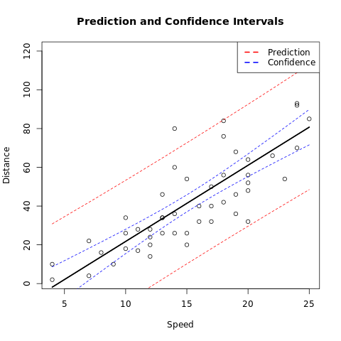
# Build the linear mod
m <- lm(dist ~ speed, data = cars)

# Create a Prediction and Confidence interval for new data on the mod
alpha <- 0.95
newdata <- list(speed = cars$speed)
make_pred <- function(type) {
    predictions = predict(m, newdata = newdata, interval = type, level = alpha)
    data.frame(speed = cars$speed, predictions)
}

# Create datafra
pred_df <- make_pred("prediction")
conf_df <- make_pred("confidence")

# Plot the Da
plot(dist ~ speed,
    data = cars,
    xlim = range(speed),
    ylim = range(dist),
    main = "Prediction and Confidence Intervals",
    xlab = "Speed",
    ylab = "Distance"
)

# Add the prediction interv
cols = c(pred = "red", conf = "blue")
with(pred_df, {
    lines(speed, fit, lwd = 2)
    lines(speed, lwr, lty = 2, col = cols["pred"])
    lines(speed, upr, lty = 2, col = cols["pred"])
})
# Add the Confidence Interv
with(conf_df, {
    lines(speed, fit, lwd = 2)
    lines(speed, lwr, lty = 2, col = cols["conf"])
    lines(speed, upr, lty = 2, col = cols["conf"])
})

## Add a lege
legend("topright",
    legend = c("Prediction", "Confidence"),
    lty = c(2, 2), col = cols, lwd = 2
)

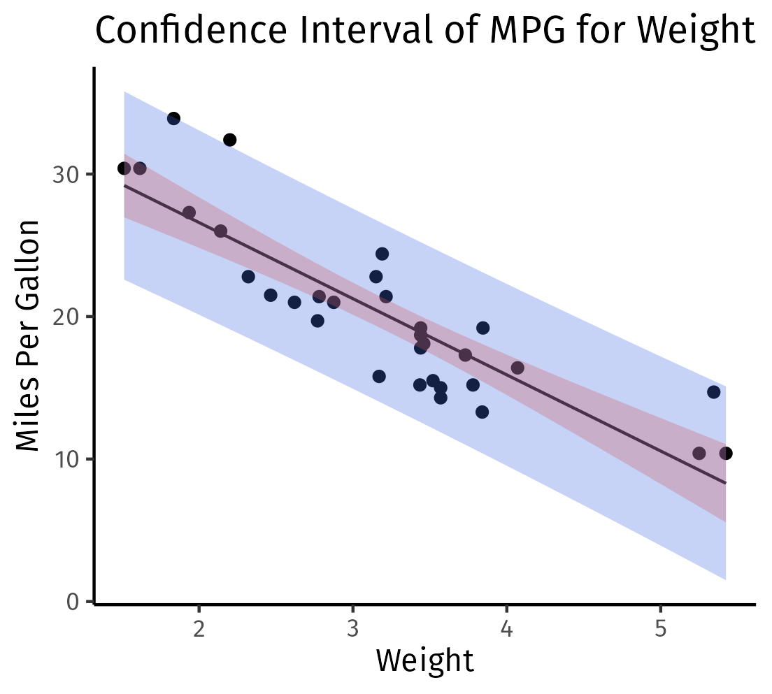
Tidyverse and GGPlot

# Load necessary librari
library(ggplot2)
library(tidyverse)
library(broom)

# Fit a linear model (Predict mpg using a single predictor, e.g., w
fit <- lm(mpg ~ wt, data=mtcars)

newdata <- data.frame(wt = seq(min(mtcars$wt), max(mtcars$wt), len=100))

conf_int <- predict(fit, newdata = newdata, interval = 'confidence') %>%
  as_tibble() %>%
  mutate(wt = newdata$wt)

pred_int <- predict(fit, newdata = newdata, interval = 'prediction') %>%
  as_tibble() %>%
  mutate(wt = newdata$wt)

# Making ggplot including confidence interv
ggplot() +
  geom_point(data = mtcars, aes(x=wt, y=mpg)) +
  geom_line(data=conf_int, aes(x=wt, y=fit)) +
  geom_ribbon(data=pred_int, aes(x = wt, y = fit, ymin=lwr, ymax=upr), alpha=0.3, fill = "royalblue") +
  geom_ribbon(data=conf_int, aes(x = wt, y = fit, ymin=lwr, ymax=upr), alpha=0.3, fill = "indianred") +
  labs(title="Confidence Interval of MPG for Weight", x="Weight", y="Miles Per Gallon") +
  theme_classic()

ggsave("../assets/images/confidence_and_prediction_interval.png")

Bootstrap

A simple bootstrap for the prediction interval of a linear model is included below. Note this assumes constant variance across the model, see ⁷ for a more detailed walkthrough of bootstrapping prediction intervals.

pred_vals <- replicate(10 ^ 4, {
  n = nrow(my_cars)
  form <- dist ~ speed
  ## Re-Sample the cars with replacement
  s = sample(1:n, replace = TRUE)
  cars_boot <- my_cars[s,]

  ## Fit a Linear Model
  mod <- lm(form, cars_boot)

  inter <- coef(mod)[1]
  slope <- coef(mod)[2]

  ## Get the predicted value at x=10
  pred_val <- 10 * slope + inter
  
  ## Find the residuals of the bootstrap model
  residuals <- resid(mod)
  
  ## Randomly select one of the residuals
  selected_resid <- sample(residuals, 1)
  
  ## Add the selected residual to the predicted value
  pred_val_selected_resid <- pred_val + selected_resid

  pred_val_selected_resid

})

hist(pred_vals)

quantile(pred_vals, c(0.025, 0.975))

## Confidence Interval
form <- dist ~ speed
fit <- lm(form, my_cars)
stats::predict(
  fit,
  newdata = list(speed = 10),
  interval = "prediction",
  levels = c(0.025, 0.975)
)

Derivation

Note

Adapted from ⁹.

We define Linear regression for matrices $X$ and $Y$ as:

$Y = BX$

The closed form solution for $X$ is:

$B = (X^{T} X)^{- 1} X^{T} Y$

We define:

Population Slope
- $β$
Sample Slope
- $B$

In the context of linear regression both $β$ and $B$ represent matrices of coefficients. If $size (Y) = n \times 1$ then the coefficient matrices will simply be vectors.

As a first step, we must solve the covariance of the weights matrix, before reading further make sure to review Covariance.

To begin, recall that the sum of variance in two vectors is the sum of the variance in each plus double the covariance:

$var (X - Y) = i = 1 \sum n [(x - y - (\overset{x}{ˉ} - \overset{y}{ˉ}))^{2}] = i = 1 \sum n [x^{2} - 2 x y + y^{2} - 2 x \overset{x}{ˉ} + 2 x \overset{y}{ˉ} + 2 \overset{x}{ˉ} y + 2 y \overset{y}{ˉ} + \overset{x}{ˉ}^{2} - 2 \overset{x}{ˉ} y + \overset{y}{ˉ}^{2}] = i = 1 \sum n [x^{2} - 2 x \overset{x}{ˉ} + \overset{x}{ˉ}^{2}] - 2 i = 1 \sum n [(x - \overset{x}{ˉ}) (y - \overset{y}{ˉ})] + i = 1 \sum n [y^{2} - 2 y \overset{y}{ˉ} + \overset{y}{ˉ}^{2}] = var (x) - 2 cov (x, y) + var (y)$

We can decompose the weights matrix to include the population weights and the noise in the observation:

$B = (X^{T} X)^{- 1} X^{T} Y = (X^{T} X)^{- 1} X^{T} (Xβ + ε) = (X^{T} X)^{- 1} X^{T} Xβ + (X^{T} X)^{- 1} X^{T} ε = (X^{T} X)^{- 1} (X^{T} X) β + (X^{T} X)^{- 1} X^{T} ε = β + (X^{T} X)^{- 1} X^{T} ε$

This can be used to show the weights matrix is an unbiased estimator of the population weights:

$E (B) = E [β + (X^{T} X)^{- 1} X^{T} ε] = E [β] + E [(X^{T} X)^{- 1} X^{T} ε] = β + (X^{T} X)^{- 1} X^{T} E [ε] The expected value of ε is 0 = β + (X^{T} X)^{- 1} X^{T} 0 = β$

Re-arranging, this gives the difference between the sample and population weights matrix:

$B - E [B] (B - E [B])^{T} = B - β = β + (X^{T} X)^{- 1} X^{T} ε - β = (X^{T} X)^{- 1} X^{T} ε = ((X^{T} X)^{- 1} X^{T} ε)^{T} = (X^{T} ε)^{T} ((X^{T} X)^{- 1})^{T} = εX ((X^{T} X)^{T})^{- 1} = εX (X^{T} X)^{- 1}$ Finally, we can solve the covariance matrix in terms of the population standard deviation: $cov (B) = E [(B - E [B]) (B - E [B])^{T}] = (X^{T} X)^{- 1} X^{T} E [ε ε^{T}] X (X^{T} X)^{- 1} = (X^{T} X)^{- 1} X^{T} σ^{2} I X (X^{T} X)^{- 1} = σ^{2} (X^{T} X)^{- 1} X^{T} X (X^{T} X)^{- 1} = σ^{2} (X^{T} X)^{- 1}$

The confidence interval depends on the variance in model predictions:

$var (\overset{y}{^}_{0}) = E [(X_{0} B - E [X_{0} B]) (X_{0} B - E [X_{0} B])^{T}] = X_{0} E [(B - E [B]) (B - E [B])^{T}] X_{0}^{T} = X_{0} cov (B) X_{0}^{T} = σ^{2} X_{0} (X^{T} X)^{- 1} X_{0}^{T}$

This is the standard error used to solve the confidence interval.

The prediction interval is the standard error in the residuals, which is given by:

$var (y_{0} - \overset{y}{^}_{0}) = var (y_{0}) - 2 cov (y_{0}, \overset{y}{^}_{0}) + var (\overset{y}{^}_{0}) = var (ε_{0}) - 2 cov (ε_{0}, \overset{y}{^}_{0}) + var (\overset{y}{^}_{0}) = var (ε_{0}) - 2 X_{0} cov (ε_{0}, B) + var (\overset{y}{^}_{0}) In Linear regression, the variance of the error is independent of the slope, so covariance is 0 = var (ε_{0}) - 0 + var (\overset{y}{^}_{0}) = σ^{2} + σ^{2} X_{0} (X^{T} X)^{- 1} X_{0}^{T} = σ^{2} (1 + X_{0} (X^{T} X)^{- 1} X_{0}^{T})$

Using this we can solve the confidence interval with:

$\overset{x}{ˉ} \pm z_{α} SE$

Of course, we don't know $σ$ so we use t, it can be shown : ¹⁰

$\frac{β - β ^}{σ ^} = \frac{N ( 0 , C ^{- 1} )}{χ _{n - p}^{2} / ( n - p )} \sim t_{n - p}$

which implies

confidence interval:

$Y \in B \pm t_{α, (n - p)} var (\hat{Y})$
prediction interval:

$Y_{i} \in B \pm t_{α, (n - p)} var (Y - \hat{Y})$

Where $C = (X^{T} X)^{- 1}$ is the control matrix.

Footnotes

⁸

https://online.stat.psu.edu/stat501/lesson/3/3.3

https://en.wikipedia.org/wiki/Prediction_interval#Estimation_of_parameters

⁵

Dunnett, C.W. (1955). A Multiple Comparisons Procedure for Comparing Several Treatments with a Control. Journal of the American Statistical Association 50, 1096-1121. cited in ¹¹

predIntNormK in https://search.r-project.org/CRAN/refmans/EnvStats/html/predIntNormK.html cited predIntNorm help page, see generally the manual Millard, Steven P. EnvStats: An R Package for Environmental Statistics. New York: Springer, 2013.

⁴

Rob J Hyndman's blog (Author of ⁷) https://robjhyndman.com/hyndsight/narrow-pi/ cited in https://joaquinamatrodrigo.github.io/skforecast/0.4.3/notebooks/prediction-intervals.html

⁷

Hyndman, Rob J., and George Athanasopoulos. Forecasting: Principles and Practice. Third print edition. Melbourne, Australia: Otexts, Online Open-Access Textbooks, 2021. https://otexts.com/fpp3/#.

⁶

Ch. 6, eq 6.22 Millard, Steven P., and Nagaraj K. Neerchal. Environmental Statistics with S-Plus. Applied Environmental Statistics. Boca Raton: CRC Press, 2001.

TODO, see generally https://en.wikipedia.org/wiki/Prediction_interval#Estimation_of_parameters

¹⁰

p. 89 § 3.7 of Bingham, N. H., and John M. Fry. Regression: Linear Models in Statistics. Springer Undergraduate Mathematics Series. London ; New York: Springer, 2010.

⁹

https://real-statistics.com/multiple-regression/confidence-and-prediction-intervals/confidence-and-prediction-intervals-proofs/

Tolerance Intervals

See 141 of EnvStats by Millard

Definition

A tolerance interval is a range that is likely to contain a specified proportion $(β 100%)$ of the population, where $β 100%$ ) is known as the coverage.

For example: Taking heights of students as an example.

Confidence Interval would be saying we are 95% confident that the population mean lies between 150cm and 200cm.

Tolerance Interval would be saying that we are 95% confident that 80% $(β 100%)$ of the individual heights in the population lies between 150cm and 200cm.

The difference is that it isn't giving the range of values for a parameter estimate, rather it is a range where a proportion of future data points are likely to lie.

Constructing Tolerance Intervals

$β$ -content tolerance interval

This is constructed so that it contains at least $β 100$ of the poulation. i.e. the coverage is at least $β 100%$ , with probability $(1 - α) 100%$ .

$β$ -expectation tolerance interval

This is constructed so that it contains on average $β 100%$ of the population.

For a Normal Distribution

For normally distributed data, the upper ( $U$ ) and lower ( $L$ ) tolerance limits are computed form a series of measurements $Y_{n}, ..., Y_{N}$

$Y_{U} = \overset{ˉ}{Y} + K_{2} s$

$Y_{L} = \overset{ˉ}{Y} - K_{2} s$

Where $K$ is the tolerance factor:

$K = t (\frac{α}{2}, n - 1) 1 + \frac{1}{n} + \frac{t ^{2} ( \frac{P}{2} , n - 1 )}{2 n}$

$P$ is the coverage ( $β 100%$ )
$t (\frac{α}{2}, n - 1)$ is the t-distribution for $a lp ha$ , the significance level
$t^{2} (\frac{P}{2}, n - 1)$ is the t-distribution for $P$ , the proportion coverage

Example in R

set.seed(222)
Y <- rnorm(100, mean=10, sd=2)

alpha <- 0.05  # significance level (95% CI)
P <- 0.85  # proportion of the population to be covered
n <- length(Y)

Ybar <- mean(Y)
s <- sd(Y)

## Calculating K tolerance factor
t_alpha <- qt(1-alpha/2, df = n-1)
t_P <- qt(1-(1-P)/2, df=n-1)

K <- t_alpha * sqrt(1 + 1/n + (t_P^2)/2/n)
U <- Ybar + K * s
L <- Ybar - K * s

print(paste("Tolerance Interval:", round(L, 4), round(U, 4)))

[1] "Tolerance Interval: 6.2033 13.8846"

Compare this with the EnvStats package

library(EnvStats)
tolIntNorm(Y, coverage=P, conf.level=1-alpha)$interval$limits

      LTL       UTL
 6.900067 13.187851

They are close but not equivalent, because the EnvStats package uses a slight different, more complicated algorithm (See ¹).

But from this, we can see that with 95% confidence, 85% of the population will lie between 6.9 and 13.2

https://rdrr.io/cran/EnvStats/src/R/tolIntNormK.R

Control Charts

Control charts are a graphical and statistical method of assessing the performance of a system over time.

They were developed in the 1920s by Walter Shewhart and have been employed widely in industry to maintain process control.

However, control charts assume the observations are independent and follow a normal distribution with some constant mean $μ$ and standard deviation $σ$

Shewhart Control Chart

A Shewhart control chart is to plot the observations over time and compare them to established upper and/or lower control limits that are based on historical data.

Once a single observation falls outside the control limit(s), this is an indication that the process is "out of control" and needs to be investigated.

$UCL = \overset{x}{ˉ} + L s$ $LCL = \overset{x}{ˉ} - L s$

The constant $L$ is often set to $L = 3$ , and the limits are called 3-sigma control limits

CUSUM Charts

To detect a gradual trend in the process, we may use Cumulative Summation (CUSUM) charts.

For the $i_{t h}$ future sampling occasion, the $i_{t h}$ upper cumulative sum $S_{i}^{+}$ and lower cumulative sum $S_{i}^{-}$

$S_{i}^{+} = max [0, (\frac{x _{i} - x ˉ}{s} - k) + S_{i - 1}^{+}], with S_{0}^{+} = 0$

$S_{i}^{-} = min [0, (\frac{x _{i} - x ˉ}{s} - k) + S_{i - 1}^{+}], with S_{0}^{-} = 0$

Where $k$ is a given positive threshold that corresponds to half the size of a linear trend (in units of standar deviations), dependent on how sensitive to detection.

With a CUSUM chart, we declare a process "out of control" when the upper/lower cumulative sums are more extreme that a pre-specified decision bound, called the decision interval. Typically this is between 4 and 5.

Example in R

## Writing out the data
month <- 1:8
## baseline values in 1995
baseline <- c(32.8, 15.2, 13.5, 39.6, 37.1, 10.4, 31.9, 20.6)
## compliance values in 1996
compliance <- c(19, 34.5, 17.8, 23.6, 34.8, 28.8, 43.7, 81.8)

nickel <- data.frame(month, baseline, compliance)

  month baseline compliance
1     1     32.8       19.0
2     2     15.2       34.5
3     3     13.5       17.8
4     4     39.6       23.6
5     5     37.1       34.8
6     6     10.4       28.8
7     7     31.9       43.7
8     8     20.6       81.8

## summary estimates from baseline
mean(baseline)
sd(baseline)

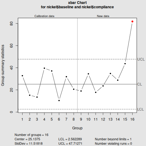
Shewhart Control Chart

library(qcc)
qcc(nickel$baseline,
    type="xbar",
    std.dev=sd(nickel$baseline),
    newdata=nickel$compliance,
    nsigmas=3,
    confidence.level=0.95)

Shewhart Control Chart

CUSUM Control Chart

cusum(nickel$baseline,
      std.dev=sd(nickel$baseline),
      decision.interval=4,
      se.shift=1,
      newdata=nickel$compliance)

Cusum Control Chart

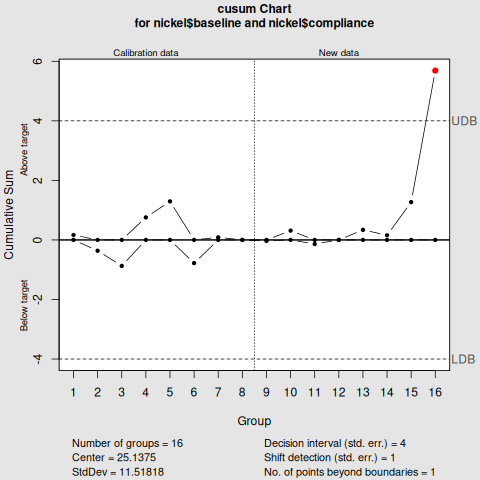
Interpretation

Notice that the key difference between the two is the nsigmas in Shewhart control chart, and the decision.interval in the cusum control chart.

From the two visualisations, month 8 exceed the upper limit, deeming the nickel concentration "out of control".

Summary

Confidence Interval gives an estimate of a population parameter
Prediction Interval predicts where a single future observation will fall
Tolerance Interval gives a cover of where a specified proportion of the poulation will fall.
Control Charts have been suggested as an alternative to prediction or tolerance intervals, for determining whether a process is in a state of statistical control.

Displaying Dates

We haven't discussed time series yet, when do, we will need to describe dates. There are countless ways to format a date but there is only one way we will do it, ISO8601 ¹. In the ISO8601 we represent dates like so:

2006-01-02T15:04:05Z07:00

This corresponds to:

Mon Jan 2 15:04:05 MST 2006

Displaying Dates

`strftime`

The more common way to format time is strftime. This approach uses a collection of symbols to represent components of time, for a list of these symbols see man strftime ², R's ?strftime and Python's help(time.strftime):

man strftime

The characters of ordinary character sequences (including the null byte) are copied verbatim from format to s.  However, the characters of conversion specifications are replaced as shown in
    the list below.  In this list, the field(s) employed from the tm structure are also shown.

    `%a`     The abbreviated name of the day of the week according to the current locale.  (Calculated from tm_wday.)  (The specific names used in the current locale can be  obtained  by  calling
           nl_langinfo(3) with ABDAY_{1–7} as an argument.)

    `%A`     The  full name of the day of the week according to the current locale.  (Calculated from tm_wday.)  (The specific names used in the current locale can be obtained by calling nl_lang‐
           info(3) with DAY_{1–7} as an argument.)

    `%b`     The abbreviated month name according to the current locale.  (Calculated from tm_mon.)  (The specific names used in the current locale can be obtained by calling nl_langinfo(3)  with
           ABMON_{1–12} as an argument.)

    `%B`     The  full  month  name  according  to  the  current  locale.  (Calculated from tm_mon.)  (The specific names used in the current locale can be obtained by calling nl_langinfo(3) with
              MON_{1–12} as an argument.)

The strftime approach was named after the C library that popularized it, it's used in C++, Rust, R, Python, PHP, Ruby and many more.

To represent in ISO8601 via strftime, the format would be %Y-%m-%dT%H:%M:%S, so e.g.:

format(Sys.time(), "%Y-%m-%dT%H:%M:%S")

Python

from datetime import datetime

now = datetime.now()
formatted = now.strftime("%Y-%m-%dT%H:%M:%S")
print(formatted)

Shell

# ISO8601
date "+%Y-%m-%dT%H:%M:%S"
# Unix
date %+s

More Languages

Rust

extern crate chrono;

use chrono::offset::Local;
use chrono::DateTime;

fn main() {
    let now: DateTime<Local> = Local::now();
    
    println!("{}", now.format("%Y-%m-%dT%H:%M:%S").to_string());
}

Julia

using Dates

println(Dates.format(now(), "yyyy-mm-ddTHH:MM:SS"))

#include <stdio.h>
#include <time.h>

int main() {
char buffer[80];
time_t t = time(NULL);
struct tm *tm_info;

tm_info = localtime(&t);
strftime(buffer, 80, "%Y-%m-%dT%H:%M:%S", tm_info);

printf("%s\n", buffer);

return 0;
}

You'll notice that each language (except Go and Julia) uses a similar approach to format the time, standardized by the strftime approach.

Reference Time

In this approach the language requires a specific date to format time, the specific date (Mon Jan 2 15:04:05 MST 2006) was a design decision made by the development team because they are distinct in the context of a date -- they used each number from 0 to 6 only once:

2006: Represents the full year format.
01: Stands for the numerical month format.
02: Represents the day of the month.
15: Stands for the 24-hour format time.
04: Represents the minutes.
05: Represents the seconds.
MST: Time zone
Mon and Jan: Are used for the abbreviated day of the week and month respectively.

Reference time is not a common approach, it's more of a unique quirk of the Go language. We draw attention to it here because it is a convenient way to express time in a human readable way, this can be useful when looking up documentaion, researching or querying a LLM. For example, to print the current time in ISO8601 format we would write it like this:

package main

import (
	"fmt"
	"time"
)

func main() {
	t := time.Now()
	fmt.Println(t.Format("2006-01-02T15:04:05-0700"))
}

Naive Forecasts

Measuring Prediction Accuracy

Roll Forward Validation

Time Series Analysis

readings

Ch. 3-5 of https://otexts.com/fpp3/decomposition.html
Ch. 2-5.3 of Shmueli, Galit, and Kenneth C. Lichtendahl. Practical Time Series Forecasting with R: A Hands-on Guide. Second edition. Erscheinungsort nicht ermittelbar: Axelrod Schnall Publishers, 2018.
3-5 of Rob J., and George Athanasopoulos. Forecasting: Principles and Practice. Third print edition. Melbourne, Australia: Otexts, Online Open-Access Textbooks, 2021. https://otexts.com/fpp3/#.
ss 1.2, 1.8, 1.11, 1.3, 1.4, 1.5, 1.14, 1.15 of tsa3

Visualisation
Time Series Decomposition
- Components (Trend, Cycle, Season)
- Classical
  - Additive
  - Multiplicative
- Decomposition by Statistical Agencies, we won't cover these
  - X-11
  - SEATS
- STL Decomposition
Autocorrelation
- ACF
- PACF
Functions in Time Series
- Mean and Variance
- Covariance
- Auto-Covariance
- Autocorrelation
Processes
- Stationary Time Series
- White Noise
- Random Walk
  - Drift
- Moving Average
- Auto Regressive
Simple Forecasting Methods
- Naive Method
- Mean Method
- Residual Diagnostics
```
google_2015 |>
  model(NAIVE(Close)) |>
  gg_tsresiduals()
```
Checklist:
- Merge old notes 06.docx
- Merge Stoffer's TSA3
- Merge Lecture Slides SP2020.pptx
  - Start with ~/Studies/Teaching/2023/Spring/Env_Info/environmental-informatics_private/New_Material/06/todo/6_Time Series and Autocorrelation (Wk 6)/Lecture 6.docx, much of the slides are built off that.
- Merge fpp3

Data Driven: Smoothing Methods

Moving Average

Exponential Smoothing

State Space Models

Model Based: ARIMA Models

Appendix

Multiple overlayed models

library(tidyverse)

## Make some data.........................................
n <- 200
x <- seq(from = -9, to = 9, length.out = n)
y_t <- exp(x) / (1 + exp(x))
y <- y_t + rnorm(n, mean = 0, sd = 0.3)
i <- sample(c(TRUE, FALSE), size = n, replace = TRUE)
data <- tibble(x, y, Set = c("train", "test")[i %% 2 + 1])

## Construct some polynomial models.......................
preds <- list()
for (i in 1:6) {
    ## [glue]
    mod <- lm(y ~ poly(x, i), filter(data, Set == "train"))
    data <- data %>%
        mutate("Deg: {i}" := predict(mod, newdata = data["x"]))
}

## Plot the data..........................................
data_tidy <- data %>%
    select(!c(y, Set)) %>%
    pivot_longer(cols = !x, names_to = "Degree")
data_tidy

ggplot(data_tidy) +
    geom_point(data = data, aes(x = x, y = y, shape = Set), size = 2) +
    geom_line(aes(x = x, y = value, color = Degree), lwd = 1) +
    geom_line(data = tibble(x, y = y_t), aes(x = x, y = y), lwd = 3) +
    theme_bw() +
    labs(x = "Input", y = "Output",
         title = "Visualisation of Model Performance")

ggsave("many_model_plot.png")


## [glue] This is glue like syntax available in dplyr>=1.

Fisher's Z Transform

get_conf_interval <- function(samp, alpha) {
    lower = (1-alpha)/2
    upper = 1-lower

    z <- make_sampling_dist(samp)

    ## z is not normally distributed, we could improve accuracy with
    ## Fisher's z-transformation
    z <- 0.5 * log((1 + z) / (1 - z))

    quantile(z, c(lower, upper))
}

Environmental Informatics (MATH3005)